The length of a coastline

This page accompanies Chapter 1 of O’Sullivan and Unwin (2010). There is only one numerical example in this chapter, and it is a complicated one. I reproduce it here anyway, perhaps you can revisit it when you reach the end of the book (and you will be amazed to see how much you have learned!).

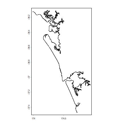
On page 13 the fractional dimension of a part of the New Zealand coastline is computed. First we get a high spatial resolution (30 m) coastline.

Throughout this book, we will use data that is installed with the rspat package. To install this package (from github) you can use the install_github function from the remotes package (so you may need to run install.packages("remotes") first.

if (!require("remotes")) install.packages("remotes")
## Loading required package: remotes

Now install rspat

if (!require("rspat")) remotes::install_github("rspatial/rspat")
## Loading required package: rspat
## Loading required package: terra
## terra 1.7.62

Now you should have the data for all chapters.

library(terra)
library(rspat)
coast <- spat_data("nz_coastline")
coast
##  class       : SpatVector
##  geometry    : lines
##  dimensions  : 1, 0  (geometries, attributes)
##  extent      : 173.9854, 174.9457, -37.47378, -36.10576  (xmin, xmax, ymin, ymax)
##  coord. ref. : +proj=longlat +ellps=WGS84 +towgs84=0,0,0,0,0,0,0 +no_defs
plot(coast)

To speed up the distance computations, we transform the CRS from longitude/latitude to a planar system.

prj <- "+proj=tmerc +lat_0=0 +lon_0=173 +k=0.9996 +x_0=1600000 +y_0=10000000 +datum=WGS84 +units=m"
mcoast <- project(coast, prj)
mcoast
##  class       : SpatVector
##  geometry    : lines
##  dimensions  : 1, 0  (geometries, attributes)
##  extent      : 1688669, 1772919, 5851165, 6003617  (xmin, xmax, ymin, ymax)
##  coord. ref. : +proj=tmerc +lat_0=0 +lon_0=173 +k=0.9996 +x_0=1600000 +y_0=10000000 +datum=WGS84 +units=m +no_defs

On to the tricky part. A function to follow the coast with a yardstick of a certain length.

Argument x is a matrix with two columns (x and y coordinates)

stickpoints <- function(x, sticklength, lonlat) {
    nr <- nrow(x)
    pts <- 1
    pt <- 0
    sticklength <- sticklength * 1000
    while(TRUE) {
        pd <- distance(x[1,], x)
        # i is the first point further than the yardstick
        i <- which(pd > sticklength)[1]
        # if we cannot find a point within yardsitck distance we
        # break out of the loop
        if (is.na(i)) break
        # remove the all points we have passed
        x <- x[(i+1):nrow(x), ]
        pt <- pt + i
        pts <- c(pts, pt)
    }
    pts
}

With this function we can compute the length of the coastline with yardsticks of different lengths.

# get the x and y coordinates of the nodes
g <- as.points(mcoast)
# reverse the order (to start at the top rather than at the bottom)
g <- rev(g)
# three yardstick lengths
sticks <- c(50, 25, 10) # km
# create an empty list for the results
y <- list()
# loop over the yardstick lengths
for (i in 1:length(sticks)) {
    y[[i]] <- stickpoints(g, sticks[i], FALSE)
}
# These last four lines are equivalent to:
# y <- lapply(sticks, function(s) stickpoints(g, s, FALSE))

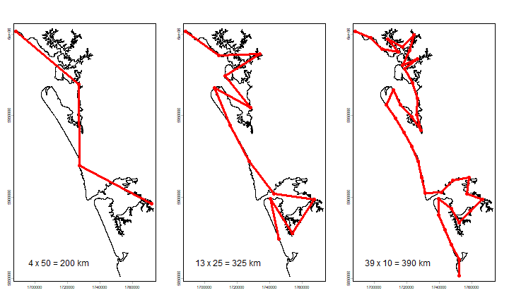
Object y has the indices of g where the stick reached the coastline. We can now make plots as in Figure 1.1. First the first three panels.

n <- sapply(y, length)
par(mfrow=c(1,3))
for (i in 1:length(y)) {
    plot(mcoast)
    stops <- y[[i]]
    points(g[stops, ], col="red", pch=20, cex=2)
    lines(g[stops, ], col="red", lwd=3)
    text(1715000, 5860000, paste(n[i], "x", sticks[i], "=", n[i] * sticks[i], "km"), cex=1.5)
}

The fractal (log-log) plot.

plot(sticks, n, log="xy", cex=3, pch=20, col="red",
    xlab="stick length", ylab="number of measures", las=1)
m <- lm(log(n) ~ log(sticks))
lines(sticks, exp(predict(m)), lwd=2, col="blue")
cf <- round(coefficients(m) , 3)
txt <- paste("log N =", cf[2], "log L +", cf[1])
text(6, 222, txt)

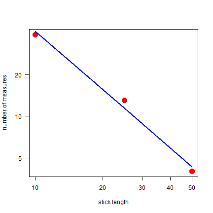
The fractal dimension D is the (absolute value of the) slope of the regression line.

-cf[2]
## log(sticks)
##       1.404

Pretty close to the 1.44 that OSU found.

Question 1: Compare the results in OSU and computed here for the three yardsticks. How and why are they different?

For a more detailed and complex example, see the fractal dimension of the coastline of Britain page.