Spatial autocorrelation
Introduction
This handout accompanies Chapter 7 in O’Sullivan and Unwin (2010).
The area of a polygon
Create a polygon like in Figure 7.2 (page 192).
library(terra)
## terra 1.9.21
pol <- matrix(c(1.7, 2.6, 5.6, 8.1, 7.2, 3.3, 1.7, 4.9, 7, 7.6, 6.1, 2.7, 2.7, 4.9), ncol=2)
sppol <- vect(pol, "polygons")
For illustration purposes, we create the “negative area” polygon as well
negpol <- rbind(pol[c(1,6:4),], cbind(pol[4,1], 0), cbind(pol[1,1], 0))
spneg <- vect(negpol, "polygons")
Now plot
cols <- c('light gray', 'light blue')
plot(sppol, xlim=c(1,9), ylim=c(1,10), col=cols[1], axes=FALSE, xlab='', ylab='',
      lwd=2, yaxs="i", xaxs="i")
plot(spneg, col=cols[2], add=T)
plot(spneg, add=T, density=8, angle=-45, lwd=1)
segments(pol[,1], pol[,2], pol[,1], 0)
text(pol, LETTERS[1:6], pos=3, col='red', font=4)
arrows(1, 1, 9, 1, 0.1, xpd=T)
arrows(1, 1, 1, 9, 0.1, xpd=T)
text(1, 9.5, 'y axis', xpd=T)
text(10, 1, 'x axis', xpd=T)
legend(6, 9.5, c('"positive" area', '"negative" area'), fill=cols, bty = "n")
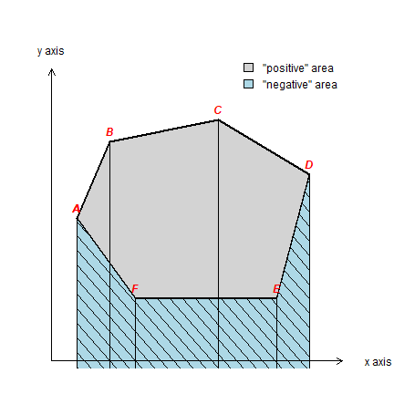
Compute area
p <- rbind(pol, pol[1,])
x <- p[-1,1] - p[-nrow(p),1]
y <- (p[-1,2] + p[-nrow(p),2]) / 2
sum(x * y)
## [1] 23.81
Or simply use an existing function. To make sure that the coordinates are not interpreted as longitude/latitude I assign an arbitrary planar coordinate reference system.
crs(sppol) <- '+proj=utm +zone=1'
expanse(sppol)
## [1] 23.68211
Contact numbers
“Contact numbers” for the lower 48 states. Get the polygons using the
geodata package:
if (!require(geodata)) remotes::install_github('rspatial/geodata')
## Loading required package: geodata
usa <- geodata::gadm(country='USA', level=1, path=".")
usa <- usa[! usa$NAME_1 %in% c('Alaska', 'Hawaii'), ]
To find adjacent polygons, we can use the relate method.
# patience, this takes a while:
wus <- relate(usa, relation="touches")
rownames(wus) <- colnames(wus) <- usa$NAME_1
wus[1:5,1:5]
##            Alabama Arizona Arkansas California Colorado
## Alabama      FALSE   FALSE    FALSE      FALSE    FALSE
## Arizona      FALSE   FALSE    FALSE       TRUE     TRUE
## Arkansas     FALSE   FALSE    FALSE      FALSE    FALSE
## California   FALSE    TRUE    FALSE      FALSE    FALSE
## Colorado     FALSE    TRUE    FALSE      FALSE    FALSE
Compute the number of neighbors for each state.
i <- rowSums(wus)
round(100 * table(i) / length(i), 1)
## i
##    1    2    3    4    5    6    7    8
##  2.0 10.2 16.3 18.4 18.4 26.5  4.1  4.1
Apparently, I am using a different data set than OSU (compare the above
with table 7.1). By changing the level argument to 2 in the
getData function you can run the same for counties.
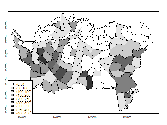
Spatial structure
Read the Auckland data from the rspat package
if (!require("rspat")) remotes::install_github('rspatial/rspat')
## Loading required package: rspat
library(rspat)
pols <- spat_data("auctb")
The tuberculosis data used here were estimated them from figure 7.7. Compare:
par(mai=c(0,0,0,0))
classes <- seq(0,450,50)
cuts <- cut(pols$TB, classes)
n <- length(classes)
cols <- rev(gray(0:n / n))
plot(pols, col=cols[as.integer(cuts)])
legend('bottomleft', levels(cuts), fill=cols)
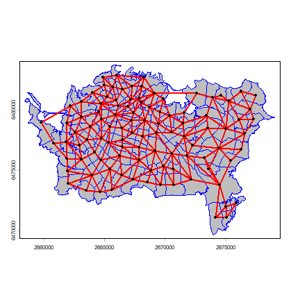
Find “rook” connetected areas.
wr <- adjacent(pols, type="rook", symmetrical=TRUE)
head(wr)
##      from to
## [1,]    1 28
## [2,]    1 53
## [3,]    1 73
## [4,]    1 74
## [5,]    1 75
## [6,]    1 76
Plot the links between the polygons.
v <- centroids(pols)
p1 <- v[wr[,1], ]
p2 <- v[wr[,2], ]
par(mai=c(0,0,0,0))
plot(pols, col='gray', border='blue')
lines(p1, p2, col='red', lwd=2)
points(v)
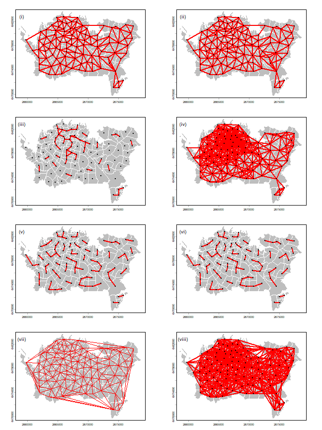
Now let’s recreate Figure 7.6 (page 202).
We already have the first one (Rook’s case adjacency, plotted above). Queen’s case adjacency:
wq <- adjacent(pols, "queen", symmetrical=TRUE)
Distance based:
wd1 <- nearby(pols, distance=1000)
wd25 <- nearby(pols, distance=2500)
Nearest neighbors:
k3 <- nearby(pols, k=3)
k6 <- nearby(pols, k=6)
Delauny:
d <- delaunay(centroids(pols))
Lag-two Rook:
wrs <- adjacent(pols, "rook", symmetrical=FALSE)
uf <- sort(unique(wrs[,1]))
wr2 <- list()
for (i in 1:length(pols)) {
    lag1 <- wrs[wrs[,1]==i, 2]
  lag2 <- wrs[wrs[,1] %in% lag1, ]
  lag2[,1] <- i
    wr2[[i]] <- unique(lag2)
}
wr2 <- do.call(rbind, wr2)
And now we plot them all using the plotit function.
plotit <- function(nb, lab='') {
  plot(pols, col='gray', border='white')
  v <- centroids(pols)
  p1 <- v[nb[,1], ]
  p2 <- v[nb[,2], ]
  lines(p1, p2, col='red', lwd=2)
  points(v)
  text(2659066, 6482808, paste0('(', lab, ')'), cex=1.25)
}
par(mfrow=c(4, 2), mai=c(0,0,0,0))
plotit(wr, 'i')
plotit(wq, 'ii')
plotit(wd1, 'iii')
plotit(wd25, 'iv')
plotit(k3, 'v')
plotit(k6, 'vi')
plot(pols, col='gray', border='white')
lines(d, col="red")
text(2659066, 6482808, '(vii)', cex=1.25)
plotit(wr2, 'viii')
Moran’s I
Below I compute Moran’s index according to formula 7.7 on page 205 of OSU.
The number of observations
n <- length(pols)
Values ‘y’ and ‘ybar’ (the mean of y).
y <- pols$TB
ybar <- mean(y)
Now we need
That is, (yi-ybar)(yj-ybar) for all pairs. I show two methods to compute that.
Method 1:
dy <- y - ybar
g <- expand.grid(dy, dy)
yiyj <- g[,1] * g[,2]
Method 2:
yi <- rep(dy, each=n)
yj <- rep(dy)
yiyj <- yi * yj
Make a matrix of the multiplied pairs
pm <- matrix(yiyj, ncol=n)
round(pm[1:6, 1:9])
##        [,1]  [,2]   [,3]   [,4]  [,5]   [,6]   [,7]   [,8]  [,9]
## [1,]  22778  4214 -12538  30776 -3181 -10727 -17821 -12387 -5445
## [2,]   4214   780  -2320   5694  -589  -1985  -3297  -2292 -1007
## [3,] -12538 -2320   6902 -16941  1751   5905   9810   6819  2997
## [4,]  30776  5694 -16941  41584 -4298 -14494 -24079 -16737 -7357
## [5,]  -3181  -589   1751  -4298   444   1498   2489   1730   760
## [6,] -10727 -1985   5905 -14494  1498   5052   8393   5834  2564
And multiply this matrix with the weights to set to zero the value for the pairs that are not adjacent.
wm <- adjacent(pols, "rook", pairs=FALSE)
wm[1:9, 1:11]
##   1 2 3 4 5 6 7 8 9 10 11
## 1 0 0 0 0 0 0 0 0 0  0  0
## 2 0 0 0 0 0 0 0 0 0  0  0
## 3 0 0 0 0 0 0 0 0 0  0  0
## 4 0 0 0 0 0 0 0 0 0  0  0
## 5 0 0 0 0 0 0 0 0 0  0  0
## 6 0 0 0 0 0 0 1 0 0  0  1
## 7 0 0 0 0 0 1 0 0 0  0  1
## 8 0 0 0 0 0 0 0 0 1  0  0
## 9 0 0 0 0 0 0 0 1 0  0  0
pmw <- pm * wm
round(pmw[1:9, 1:11])
##   1 2 3 4 5    6    7    8    9 10    11
## 1 0 0 0 0 0    0    0    0    0  0     0
## 2 0 0 0 0 0    0    0    0    0  0     0
## 3 0 0 0 0 0    0    0    0    0  0     0
## 4 0 0 0 0 0    0    0    0    0  0     0
## 5 0 0 0 0 0    0    0    0    0  0     0
## 6 0 0 0 0 0    0 8393    0    0  0  6616
## 7 0 0 0 0 0 8393    0    0    0  0 10990
## 8 0 0 0 0 0    0    0    0 2961  0     0
## 9 0 0 0 0 0    0    0 2961    0  0     0
We sum the values, to get this bit of Moran’s I:
spmw <- sum(pmw)
spmw
## [1] 1523422
The next step is to divide this value by the sum of weights. That is easy.
smw <- sum(wm)
sw  <- spmw / smw
And compute the inverse variance of y
vr <- n / sum(dy^2)
The final step to compute Moran’s I
MI <- vr * sw
MI
## [1] 0.2643226
After doing this ‘by hand’, now let’s use the terra package to compute Moran’s I.
autocor(y, wm)
## [1] 0.2643226
This is how you can (theoretically) estimate the expected value of Moran’s I. That is, the value you would get in the absence of spatial autocorrelation. Note that it is not zero for small values of n.
  EI <- -1/(n-1)
EI
## [1] -0.009803922
So is the value we found significant, in the sense that is it not a
value you would expect to find by random chance? Significance can be
tested analytically (see spdep::moran.test) but it is much better to
use Monte Carlo simulation. We test the (one-sided) probability of
getting a value as high as the observed I.
I <- autocor(pols$TB, wm)
nsim <- 99
mc <- sapply(1:nsim, function(i) autocor(sample(pols$TB), wm))
P <- 1 - sum((I > mc) / (nsim+1))
P
## [1] 0.01
Question 1: How do you interpret these results (the significance tests)?
Question 2: What would a good value be for ``nsim``?
Question 3: *Show a figure similar to Figure 7.9 in OSU.
To make a Moran scatter plot we first get the neighbouring values for each value.
n <- length(pols)
ms <- cbind(id=rep(1:n, each=n), y=rep(y, each=n), value=as.vector(wm * y))
Remove the zeros
ms <- ms[ms[,3] > 0, ]
And compute the average neighbour value
ams <- aggregate(ms[,2:3], list(ms[,1]), FUN=mean)
ams <- ams[,-1]
colnames(ams) <- c('y', 'spatially lagged y')
head(ams)
##     y spatially lagged y
## 1 271           135.1429
## 2 148           154.3333
## 3  37           142.2500
## 4 324           142.6250
## 5  99            71.6250
## 6  49            14.5000
Finally, the plot.
plot(ams)
reg <- lm(ams[,2] ~ ams[,1])
abline(reg, lwd=2)
abline(h=mean(ams[,2]), lt=2)
abline(v=ybar, lt=2)
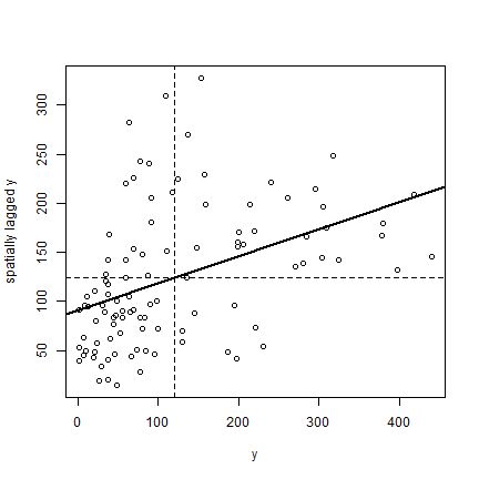
Note that the slope of the regression line:
coefficients(reg)[2]
##  ams[, 1]
## 0.2746281
is almost the same as Moran’s I.
See spdep::moran.plot for a more direct approach to accomplish the
same thing (but hopefully the above makes it clearer how this is
actually computed).
Question 4: compute Geary’s C for these data