2. The length of a coastline¶

How Long Is the Coast of Britain? Statistical Self-Similarity and Fractional Dimension is the title of a famous paper by Benoît Mandelbrot. Mandelbrot uses data from a paper by Lewis Fry Richardson who showed that the length of a coastline changes with scale, or, more precisely, with the length (resolution) of the measuring stick (ruler) used. Mandelbrot discusses the fractal dimension D of such lines. D is 1 for a straight line, and higher for more wrinkled shapes. For the west coast of Britain, Mandelbrot reports that D=1.25. Here I show how to measure the length of a coast line with rulers of different length and how to compute a fractal dimension.

First we get a high spatial resolution (30 m) coastline for the United Kingdom from the GADM database.

library(terra)
## terra 1.7.62
library(geodata)
w <- world(path=".", resolution = 3)
uk <- w[w$GID_0=="GBR", ]
plot(uk)

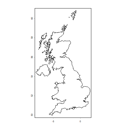
This is a single “multi-polygon” (it has a single geometry) and a longitude/latitude coordinate reference system.

as.data.frame(uk)
##   GID_0         NAME_0
## 1   GBR United Kingdom

Let’s transform this to a planar coordinate system. That is not required, but it will speed up computations. We used the British National Grid coordinate reference system, which is based on the Transverse Mercator (tmerc) projection, with units in meter.

prj <- "epsg:27700"

With that we can transform the coordinates of uk from longitude latitude to the British National Grid.

guk <- project(uk, prj)

We only want the main island, so want need to separate (disaggregate) the different polygons.

duk <- disagg(guk)
head(duk)
##   GID_0         NAME_0
## 1   GBR United Kingdom
## 2   GBR United Kingdom
## 3   GBR United Kingdom
## 4   GBR United Kingdom
## 5   GBR United Kingdom
## 6   GBR United Kingdom

Now we have 920 features. We want the largest one.

a <- expanse(duk)
i <- which.max(a)
a[i] / 1000000
## [1] 219769.8
b <- duk[i,]

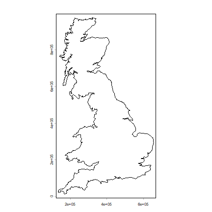
Britain has an area of about 220,000 km².

par(mai=rep(0,4))
plot(b)

On to the tricky part. The function to go around the coast with a ruler (yardstick) of a certain length.

measure_with_ruler <- function(pols, stick_length, lonlat=FALSE) {
    # some sanity checking
    stopifnot(inherits(pols, "SpatVector"))
    stopifnot(length(pols) == 1)
    # get the coordinates of the polygon
    g <- geom(pols)[, c('x', 'y')]
    nr <- nrow(g)
    # we start at the first point
    pts <- 1
    newpt <- 1
    while(TRUE) {
        # start here
        p <- newpt
        # order the points
        j <- p:(p+nr-1)
        j[j > nr] <- j[j > nr] - nr
        gg <- g[j,]
        # compute distances
        pd <- distance(gg[1,,drop=FALSE], gg, lonlat)
        pd <- as.vector(pd)
        # get the first point that is past the end of the ruler
        # this is precise enough for our high resolution coastline
        i <- which(pd > stick_length)[1]
        if (is.na(i)) {
            stop('Ruler is longer than the maximum distance found')
        }
        # get the record number for new point in the original order
        newpt <- i + p
        # stop if past the last point
        if (newpt >= nr) break
        pts <- c(pts, newpt)
    }
    # add the last (incomplete) stick.
    pts <- c(pts, 1)
    # return the locations
    g[pts, ]
}

Now we have the function, life is easy, we just call it a couple of times, using rulers of different lengths (although it takes a while to run).

y <- list()
rulers <- c(25,50,100,150,200,250) # km
for (i in 1:length(rulers)) {
    y[[i]] <- measure_with_ruler(b, rulers[i]*1000)
}

Object y is a list of matrices containing the locations where the ruler touched the coast. We can plot these on top of the map of Britain.

par(mfrow=c(2,3), mai=rep(0,4))
for (i in 1:length(y)) {
    plot(b, col='lightgray', lwd=2)
    p <- y[[i]]
    lines(p, col='red', lwd=3)
    points(p, pch=20, col='blue', cex=2)
    bar <- rbind(cbind(525000, 900000), cbind(525000, 900000-rulers[i]*1000))
    lines(bar, lwd=2)
    points(bar, pch=20, cex=1.5)
    text(525000, mean(bar[,2]), paste(rulers[i], '  km'), cex=1.5)
    text(525000, bar[2,2]-50000, paste0('(', nrow(p), ')'), cex=1.25)
}

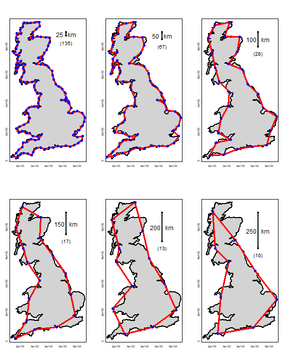
The coastline of Britain, measured with rulers of different lengths. The number of segments is in parenthesis. f

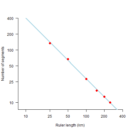
Here is the fractal (log-log) plot. Note how the axes are on the log scale, but that I used the non-transformed values for the labels.

# number of times a ruler was used
n <- sapply(y, nrow)
# set up empty plot
plot(log(rulers), log(n), type='n', xlim=c(2,6), ylim=c(2,6), axes=FALSE,
       xaxs="i",yaxs="i", xlab='Ruler length (km)', ylab='Number of segments')
# axes
tics <- c(1,10,25,50,100,200,400)
axis(1, at=log(tics), labels=tics)
axis(2, at=log(tics), labels=tics, las=2)
# linear regression line
m <- lm(log(n)~log(rulers))
abline(m, lwd=3, col='lightblue')
# add observations
points(log(rulers), log(n), pch=20, cex=2, col='red')

What does this mean? Let’s try some very small rulers, from 1 mm to 10 m.

small_rulers <- c(0.000001, 0.00001, 0.0001, 0.001, 0.01)  # km
nprd <- exp(predict(m, data.frame(rulers=small_rulers)))
coast <- nprd * small_rulers
plot(small_rulers, coast, xlab='Length of ruler', ylab='Length of coast', pch=20, cex=2, col='red')

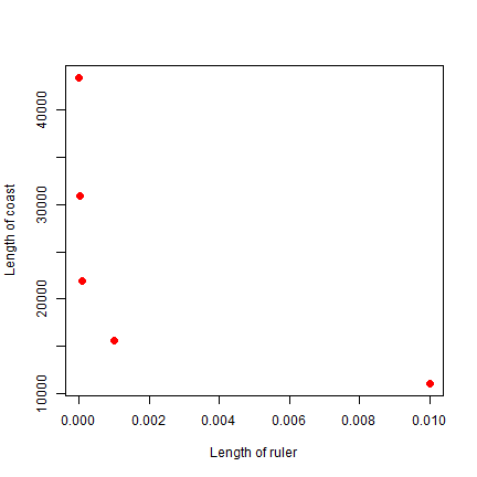
So as the ruler get smaller, the coastline gets exponentially longer. As the ruler approaches zero, the length of the coastline approaches infinity.

The fractal dimension D of the coast of Britain is the (absolute value of the) slope of the regression line.

m
##
## Call:
## lm(formula = log(n) ~ log(rulers))
##
## Coefficients:
## (Intercept)  log(rulers)
##       8.632       -1.148

Get the slope

-1 * m$coefficients[2]
## log(rulers)
##    1.148083

Not to far away from Mandelbrot’s D = 1.25 for the west coast of Britain.