Fields
Introduction
This handout accompanies Chapter 9 in O’Sullivan and Unwin (2010).
Here is how you can set up and use the continuous function on page 246.
z <- function(x, y) { -12 * x^3 + 10 * x^2 * y - 14 * x * y^2 + 25 * y^3 + 50 }
z(.5, 0.8)
## [1] 58.82
Function zf adds some complexity to make it usable in the
‘interpolate’ function below.
zf <- function(model, xy) {
   x <- xy[,1]
   y <- xy[,2]
   z(x, y)
}
Now use it
library(terra)
## terra 1.9.21
r <- rast(xmin=0.5, xmax=1.4, ymin=0.6, ymax=1.5, ncol=9, nrow=9, crs="")
z <- interpolate(r, model=NULL, fun=zf)
names(z) <- 'z'
vt <- persp(z, theta=30, phi=30, ticktype='detailed', expand=.8)
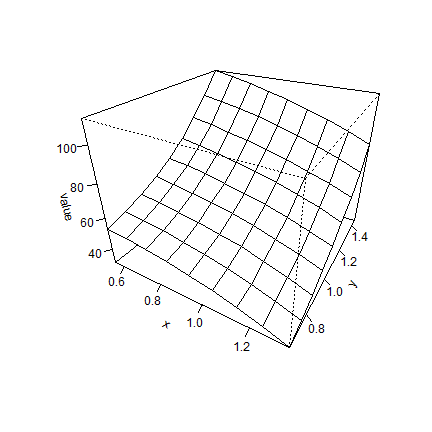
Note that persp returned something invisibly (it won’t be printed when
not captured as a variable, vt, in this case), the 3D transformation
matrix that we use later. This is not uncommon in R. For example
hist and barplot have similar behaviour.
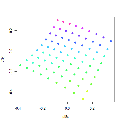
pts <- as.data.frame(z, xy=TRUE)
pt <- trans3d(pts[,1], pts[,2], pts[,3], vt)
plot(pt, col=rainbow(9, .75, start=.2)[round(pts[,3]/10)-2], pch=20, cex=2)
For a more interactive experience, try:
library(rasterVis)
library(rgl)
# this opens a new window
plot3D(raster::raster(z), zfac=5)
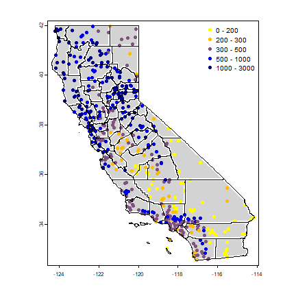
We will be working with temperature data for California. You can download the climate data used in the examples.
library(rspat)
d <- spat_data("precipitation")
head(d)
## ID NAME LAT LONG ALT JAN FEB MAR APR MAY JUN JUL
## 1 ID741 DEATH VALLEY 36.47 -116.87 -59 7.4 9.5 7.5 3.4 1.7 1.0 3.7
## 2 ID743 THERMAL/FAA AIRPORT 33.63 -116.17 -34 9.2 6.9 7.9 1.8 1.6 0.4 1.9
## 3 ID744 BRAWLEY 2SW 32.96 -115.55 -31 11.3 8.3 7.6 2.0 0.8 0.1 1.9
## 4 ID753 IMPERIAL/FAA AIRPORT 32.83 -115.57 -18 10.6 7.0 6.1 2.5 0.2 0.0 2.4
## 5 ID754 NILAND 33.28 -115.51 -18 9.0 8.0 9.0 3.0 0.0 1.0 8.0
## 6 ID758 EL CENTRO/NAF 32.82 -115.67 -13 9.8 1.6 3.7 3.0 0.4 0.0 3.0
## AUG SEP OCT NOV DEC
## 1 2.8 4.3 2.2 4.7 3.9
## 2 3.4 5.3 2.0 6.3 5.5
## 3 9.2 6.5 5.0 4.8 9.7
## 4 2.6 8.3 5.4 7.7 7.3
## 5 9.0 7.0 8.0 7.0 9.0
## 6 10.8 0.2 0.0 3.3 1.4
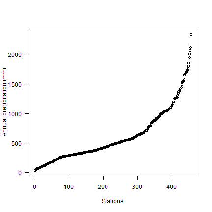
d$prec <- rowSums(d[, c(6:17)])
plot(sort(d$prec), ylab='Annual precipitation (mm)', las=1, xlab='Stations')
dsp <- vect(d, c("LONG", "LAT"), crs= "+proj=longlat +datum=WGS84")
CA <- spat_data("counties")
cuts <- c(0,200,300,500,1000,3000)
blues <- colorRampPalette(c('yellow', 'orange', 'blue', 'dark blue'))
plot(CA, col="light gray", lwd=4, border="white")
plot(dsp, "prec", breaks=cuts, col=blues(5), pch=20, cex=1.5, add=TRUE, plg=list(x="topright"))
lines(CA, lwd=1.5)