Map overlay
Introduction
This document shows some example R code to do “overlays” and associated spatial data manipulation to accompany Chapter 11 in O’Sullivan and Unwin (2010). You have already seen many of this type of data manipulation in previous labs. And we have done perhaps more advanced things using regression type models (including LDA and RandomForest). This chapter is very much a review of what you have already seen: basic spatial data operations with R.
Get the data
You can get the data for this tutorial with the “rspat” package that you can install with the line below.
if (!require("rspat")) remotes::install_github('rspatial/rspat')
## Loading required package: rspat
## Loading required package: terra
## terra 1.9.21
Selection by attribute
By now, you are well aware that in R, polygons and their attributes
can be represented by a SpatVector. Here we use a SpatVector of
California counties.
library(terra)
library(rspat)
counties <- spat_data('counties')
Selecting rows (geometries and their attributes) of a SpatVector is
similar to selecting rows from a data.frame. For example, to select
Yolo county by its name:
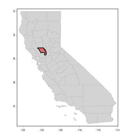
yolo <- counties[counties$NAME == 'Yolo', ]
plot(counties, col='light gray', border='gray')
plot(yolo, add=TRUE, density=20, lwd=2, col='red')
You can interactively select counties this way by clicking on the map of the counties:
plot(counties)
s <- sel(counties)
Intersection and buffer
I want to get the railroads in the city of Davis by sub-setting the railroads in Yolo county. First read the data, and do an important sanity check: are the coordinate reference systems (crs) for the two datasets the same?
rail <- spat_data("yolo-rail")
rail
## class       : SpatVector
## geometry    : lines
## dimensions  : 4, 1  (geometries, attributes)
## extent      : -122.0208, -121.5089, 38.31305, 38.9255  (xmin, xmax, ymin, ymax)
## coord. ref. : +proj=longlat +datum=WGS84 +no_defs
## names       :               FULLNAME
## type        :                  <chr>
## values      :           Abandoned RR
##               California Northern RR
##                     Union Pacific RR
##               ...
class(rail)
## [1] "SpatVector"
## attr(,"package")
## [1] "terra"
city <- spat_data("city")
crs(yolo, TRUE)
## [1] "+proj=longlat +datum=WGS84 +no_defs"
crs(rail, TRUE)
## [1] "+proj=longlat +datum=WGS84 +no_defs"
crs(city, TRUE)
## [1] "+proj=lcc +lat_0=37.6666666666667 +lon_0=-122 +lat_1=38.3333333333333 +lat_2=39.8333333333333 +x_0=2000000 +y_0=500000.000000001 +datum=WGS84 +units=us-ft +no_defs"
Ay, we are dealing with two different coordinate reference systems (projections)! Let’s settle for yet another one: Teale Albers. This is a short name for the “Albers Equal Area projection with parameters suitable for California”. This particular set of parameters was used by an California State organization called the Teale Data Center, hence the name.
TA <- "+proj=aea +lat_1=34 +lat_2=40.5 +lat_0=0 +lon_0=-120 +x_0=0 +y_0=-4000000 +datum=WGS84 +units=m"
countiesTA <- project(counties, TA)
yoloTA <- project(yolo, TA)
railTA <- project(rail, TA)
cityTA <- project(city, TA)
Another check, let’s see what county Davis is in, using two approaches. In the first one we get the centroid of Davis and do a point-in-polygon query.
davis <- centroids(cityTA)
i <- which(relate(davis, countiesTA, "intersects"))
countiesTA$NAME[i]
## [1] "Yolo"
An alternative approach is to intersect the two polygon SpatVectors
i <- intersect(cityTA, countiesTA)
i$area <- expanse(i)
as.data.frame(i)
##   STATE COUNTY   NAME LSAD LSAD_TRANS        area
## 1    06    095 Solano   06     County    78791.82
## 2    06    113   Yolo   06     County 25633905.73
plot(cityTA, col='blue')
plot(yoloTA, add=TRUE, border='red', lwd=3)
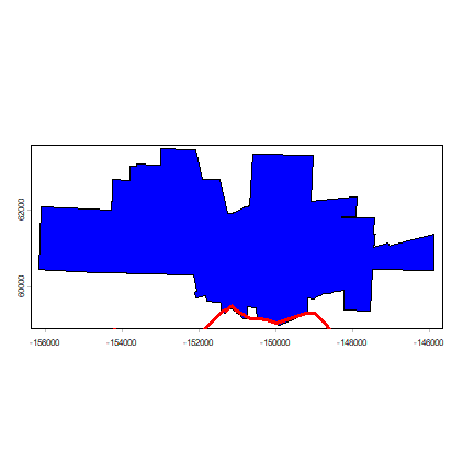
Our data suggest that we have a little sliver of Davis inside of Solano county (the county to the south of Yolo) — but that is probably not correct. At least it would seem likely that the boundaries may be the same in reality.
Otherwise, everything looks OK. Now we can intersect rail and city, and make a buffer.
davis_rail <- intersect(railTA, cityTA)
Compute a 500 meter buffer around railroad inside Davis:
buf <- buffer(railTA, width=500)
buf <- aggregate(buf)
rail_buf <- intersect(buf, cityTA)
plot(cityTA, col='light gray')
plot(rail_buf, add=TRUE, col='light blue', border='light blue')
plot(railTA, add=TRUE, lty=2, lwd=6)
plot(cityTA, add=TRUE)
plot(davis_rail, add=TRUE, col='red', lwd=6)
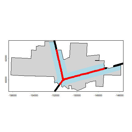
What is the percentage of the area of the city of Davis that is within 500 m of a railroad?
round(100 * expanse(rail_buf) / expanse(cityTA))
## [1] 31
Proximity
Which park in Davis is furthest, and which is closest to the railroad? First get the parks data.
parks <- spat_data("parks")
crs(parks, TRUE)
## [1] "+proj=lcc +lat_0=37.6666666666667 +lon_0=-122 +lat_1=38.3333333333333 +lat_2=39.8333333333333 +x_0=2000000 +y_0=500000.000000001 +datum=WGS84 +units=us-ft +no_defs"
parksTA <- project(parks, TA)
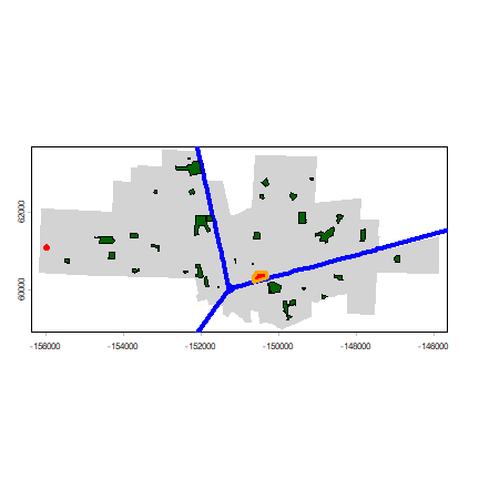
Now plot the parks that are the furthest and the nearest from a railroad.
plot(cityTA, col="light gray", border="light gray")
plot(railTA, add=TRUE, col="blue", lwd=4)
plot(parksTA, col="dark green", add=TRUE)
d <- distance(parksTA, railTA)
dmin <- apply(d, 1, min)
parksTA$railDist <- dmin
i <- which.max(dmin)
as.data.frame(parksTA)[i,]
##              PARK     PARKTYPE            ADDRESS railDist
## 26 Whaleback Park NEIGHBORHOOD 1011 MARINA CIRCLE 4330.938
plot(parksTA[i, ], add=TRUE, col="red", lwd=3, border="red")
j <- which.min(dmin)
as.data.frame(parksTA)[j,]
##                    PARK     PARKTYPE         ADDRESS railDist
## 14 Toad Hollow Dog Park NEIGHBORHOOD 1919 2ND STREET 23.83512
plot(parksTA[j, ], add=TRUE, col="red", lwd=3, border="orange")
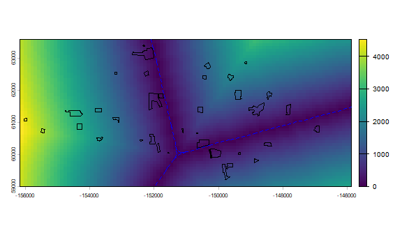
Another way to approach this is to first create a raster with distance to the railroad values. Here we compute the average distance to any place inside the park. You could also compute the distance to the border or the centroids of the parks.
# use cityTA to set the geographic extent
r <- rast(cityTA)
# arbitrary resolution
dim(r) <- c(50, 100)
# rasterize the railroad lines
r <- rasterize(railTA, r)
# compute distance
d <- distance(r)
names(d) <- "dist"
# extract distance values for polygons
dp <- extract(d, parksTA, fun=mean, exact=TRUE)
dp <- data.frame(park=parksTA$PARK, distance=dp[,2])
dp <- dp[order(dp$distance), ]
plot(d)
plot(parksTA, add=TRUE)
plot(railTA, add=T, col="blue", lty=2)
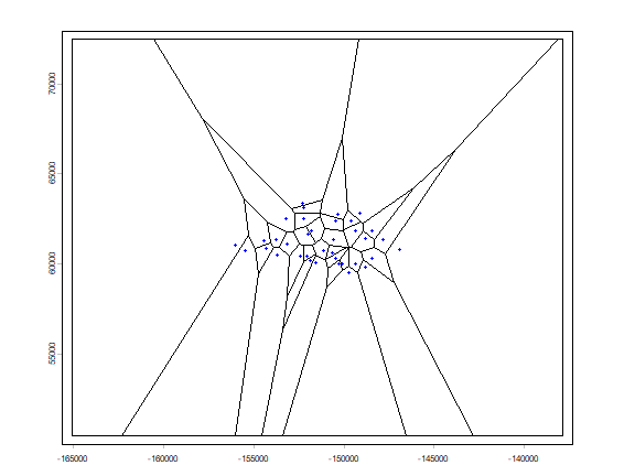
Voronoi polygons
Here I compute Voronoi (or Thiessen) polygons for the centroids of the Davis parks. Each polygon shows the area that is closest to (the centroid of) a particular park.
centr <- centroids(parksTA)
v <- voronoi(centr)
plot(v)
points(centr, col="blue", pch=20)
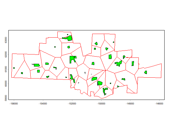
To keep the polygons within Davis.
vc <- intersect(v, cityTA)
plot(vc, border="red")
plot(parksTA, add=T, col="green")
Raster data
raster data can be read with the rast method. See the terra package
for more details
alt <- spat_data("elevation")
alt
## class       : SpatRaster
## size        : 239, 474, 1  (nrow, ncol, nlyr)
## resolution  : 0.008333333, 0.008333333  (x, y)
## extent      : -123.95, -120, 37.3, 39.29167  (xmin, xmax, ymin, ymax)
## coord. ref. : +proj=longlat +datum=WGS84 +no_defs
## source(s)   : memory
## name        : lyr.1
## min value   :   -30
## max value   :  2963
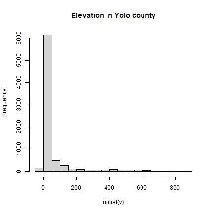
Query
Now extract elevation data for Yolo county.
v <- extract(alt, yolo)
hist(unlist(v), main="Elevation in Yolo county")
Another approach:
# cut out a rectangle (extent) of Yolo
yalt <- crop(alt, yolo)
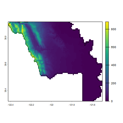
# "mask" out the values outside Yolo
ymask <- mask(yalt, yolo)
# summary of the raster cell values
summary(ymask)
## lyr.1
## Min. : -1.0
## 1st Qu.: 6.0
## Median : 28.0
## Mean :111.3
## 3rd Qu.:110.0
## Max. :882.0
## NA's :3972
plot(ymask)
plot(yolo, add=T)
You can also get values (query) by clicking on the map (use
click(alt))
Exercise
We want to travel by train in Yolo county and we want to get as close as possible to a hilly area; whenever we get there we’ll jump from the train. It turns out that the railroad tracks are not all connected, we will ignore that inconvenience.
Define “hilly” as some vague notion of a combination of high elevation and slope (in degrees). Use some of the functions you have seen above, as well as function ‘distance’ to create a plot of distance from the railroad against hillyness. Make a map to illustrate the result, showing where you get off the train, where you go to, and what the elevation and slope profile would be if you follow the shortest (as the crow flies) path.
Bonus: use the costDist function to find the least-cost path between
these two points (assign a cost to slope, perhaps using Tobler’s hiking
function).