Fundamentals
Processes and patterns
This handout accompanies Chapter 4 in O’Sullivan and Unwin
(2010)
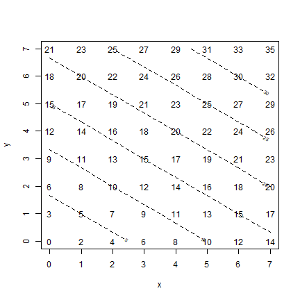
by working out the examples in R. Figure 4.2 (on page 96) shows values
for a deterministic spatial process z = 2x + 3y. Below are two ways to
create such a plot in R. The first one uses “base” R. That is, it
does not use explicitly spatial objects (classes). I use the expand.grid
function to create a matrix with two columns with all combinations of
0:7 with 0:7:
x <- 0:7
y <- 0:7
xy <- expand.grid(x, y)
colnames(xy) <- c("x", "y")
head(xy)
##   x y
## 1 0 0
## 2 1 0
## 3 2 0
## 4 3 0
## 5 4 0
## 6 5 0
Now we can use these values to compute the values of z that
correspond to the values of x (the first column of object xy)
and y (the second column).
z <- 2*xy[,1] + 3*xy[,2]
zm <- matrix(z, ncol=8)
Here I do the same thing, but using a function of my own making
(called detproc); just to get used to the idea of writing and using
your own functions.
detproc <- function(x, y) {
  z <- 2*x + 3*y
  return(z)
}
v <- detproc(xy[,1], xy[,2])
zm <- matrix(v, ncol=8)
Below, I use a trick plot(x, y, type="n") to set up a plot with the
correct axes, that is otherwise blank. I do this because I do not want
any dots on the plot. Instead of showing dots, I use the ‘text’ function
to add the labels (as in the book).
plot(x, y, type="n")
text(xy[,1], xy[,2], z)
contour(x, y, zm, add=TRUE, lty=2)
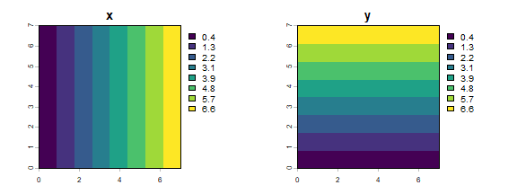
Now, let’s do the same thing as above, but now by using a spatial data
approach. Instead of a matrix, we use SpatRasters. First we create an
empty raster with eight rows and columns, and with x and y coordinates
going from 0 to 7. The init function sets the values of the cells to
either the x or the y coordinate (or something else, see ?init).
library(terra)
## terra 1.9.21
r <- rast(xmin=0, xmax=7, ymin=0, ymax=7, ncol=8, nrow=8)
X <- init(r, "x")
Y <- init(r, "y")
par(mfrow=c(1,2))
plot(X, main="x")
plot(Y, main="y")
We can use algebraic expressions with SpatRasters
Z <- 2*X + 3*Y
Do you think it is possible to do Z <- detproc(X, Y)? (try
it).
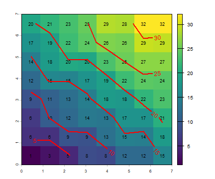
Plot the result.
plot(Z)
text(Z, cex=.75)
contour(Z, add=TRUE, labcex=1, lwd=2, col="red")
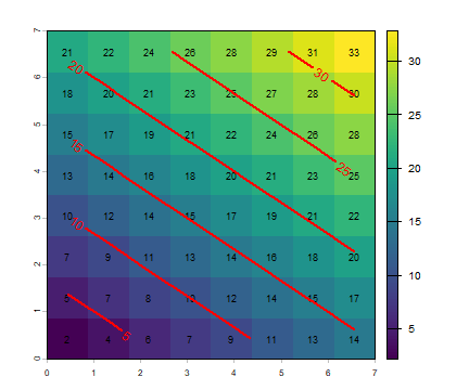
The above does not seem very interesting. But, if the process is complex, a map of the outcome of a deterministic process can actually be very interesting. For example, in ecology and associated sciences there are many “mechanistic” (= process) models that dynamically (= over time) simulate ecosystem processes such as vegetation dynamics and soil greenhouse gas emissions that depend on interaction of the weather, soil type, genotypes, and management; making it hard to predict the model outcome over space. In this context, stochasticity still exists through the input variables such as rainfall. Many other models exist that have a deterministic and stochastic components (for example, global climate models).
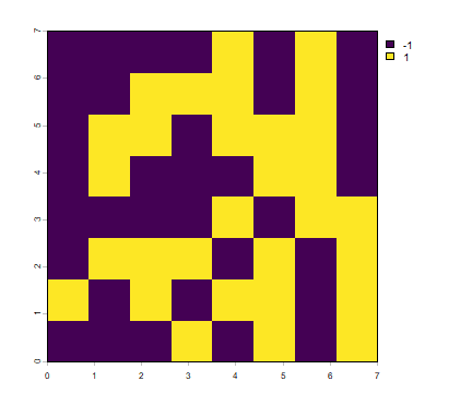
Below I follow the book by adding a stochastic element to the
deterministic process by adding variable r to the equation:
z = 2x + 3y + r; where r is a random value that can be -1 or +1.
Many examples in R manuals use randomly generated values to illustrate
how a particular function work. But much real data analysis also depends
on randomly selected variables, for example, to create a “null model”
(such as CSR) to compare with an observed data set.
There are different ways to get random numbers, and you should pay
attention to that. The sample function returns randomly selected
values from a set that you provide (by default this is done without
replacement). We need a random value for each cell of SpatRaster r,
and assign these to a new SpatRaster with the same properties (spatial
extent and resolution). When you work with random values, the results
will be different each time you run some code (that is the point); but
sometimes it is desireable to recreate exactly the same random sequence.
The function set.seed allows you to do that — to create the same
random sequence over and over again.
set.seed(987)
s <- sample(c(-1, 1), ncell(r), replace=TRUE)
s[1:8]
## [1] -1 -1 -1 -1  1 -1  1 -1
R <- setValues(r, s)
plot(R)
Now we can solve the formula and look at the result
Z <- 2*X + 3*Y + R
plot(Z)
text(Z, cex=.75)
contour(Z, add=T, labcex=1, lwd=2, col="red")
The figure above is a pattern from a (partly) random process. The process can generate other patterns, as is shown below. Because we want to repeat the same thing (process, code) a number of times, it is convenient to define a (pattern generating) function.
f <- function() {
    s <- sample(c(-1, 1), ncell(r), replace=TRUE)
    S <- setValues(r, s)
    Z <- 2*X + 3*Y + S
    return(Z)
}
We can call function f as many times as we like, below I use it four
times. Note that the function has no arguments, but we still need to use
the parenthesis f() to distinguish it from f, which is the
function itself.
set.seed(777)
par(mfrow=c(2,2), mai=c(0.5,0.5,0.5,0.5))
for (i in 1:4) {
    pattern <- f()
    plot(pattern)
    text(pattern, cex=.75)
    contour(pattern, add=TRUE, labcex=1, lwd=2, col="red")
}
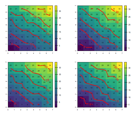
As you can see, there is variation between the four plots, but not much. The deterministic process has an overriding influence as the random component only adds or subtracts a value of 1.
So far we have created regular, gridded, patterns. Locations of “events”
normally do not follow such a pattern (but they may be summarized that
way). Here is how you can create simple dot maps of random events
(following box “All the way: a chance map”; OSU page 98). I first create
a function for a complete spatial random (CSR) process. Note the use of
the runif (pronounced as “r unif” as it stands for “random uniform”,
there is also a rnorm, rpois, …) function to create the x and y
coordinates. For convenience, this function also plots the value. That
is not typical, as in many cases you may want to create many random
draws, but not plot them all. Therefore I added the logical argument
“plot” (with default value FALSE) to the function.
csr <- function(n, r=99, plot=FALSE) {
    x <- runif(n, max=r)
    y <- runif(n, max=r)
    if (plot) {
        plot(x, y, xlim=c(0,r), ylim=c(0,r))
    }
}
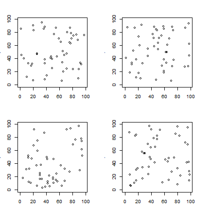
Let’s run the function four times; to create four realizations. Again, I
use set.seed to assure that the maps are always the same “random”
draws.
set.seed(0)
par(mfrow=c(2,2), mai=c(.5, .5, .5, .5))
for (i in 1:4) {
    csr(50, plot=TRUE)
}
Predicting patterns
I first show how you can recreate Table 4.1 with R. Note the use of
function choose to get the “binomial coefficients” from this
formula.
Everything else is just basic math.
events <- 0:10
combinations <- choose(10, events)
prob1 <- (1/8)^events
prob2 <- (7/8)^(10-events)
Pk <- combinations * prob1 * prob2
d <- data.frame(events, combinations, prob1, prob2, Pk)
round(d, 8)
##    events combinations      prob1     prob2         Pk
## 1       0            1 1.00000000 0.2630756 0.26307558
## 2       1           10 0.12500000 0.3006578 0.37582225
## 3       2           45 0.01562500 0.3436089 0.24160002
## 4       3          120 0.00195312 0.3926959 0.09203810
## 5       4          210 0.00024414 0.4487953 0.02300953
## 6       5          252 0.00003052 0.5129089 0.00394449
## 7       6          210 0.00000381 0.5861816 0.00046958
## 8       7          120 0.00000048 0.6699219 0.00003833
## 9       8           45 0.00000006 0.7656250 0.00000205
## 10      9           10 0.00000001 0.8750000 0.00000007
## 11     10            1 0.00000000 1.0000000 0.00000000
sum(d$Pk)
## [1] 1
Table 4.1 explains how value for the binomial distribution can be computed. As this is a “well-known” distribution (after all, it is the distribution you get when tossing a fair coin) there is a function to compute this directly.
b <- dbinom(0:10, 10, 1/8)
round(b, 8)
##  [1] 0.26307558 0.37582225 0.24160002 0.09203810 0.02300953 0.00394449
##  [7] 0.00046958 0.00003833 0.00000205 0.00000007 0.00000000
Similar functions exists for other commonly used distributions such as the uniform, normal, and Poisson distribution.
Now generate some quadrat counts and then compare the generated (observed) frequencies with the theoretical expectation. First the random points.
set.seed(1234)
x <- runif(50) * 99
y <- runif(50) * 99
And the quadrats.
r <- rast(xmin=0, xmax=99, ymin=0, ymax=99, ncol=10, nrow=10)
quads <- as.polygons(r)
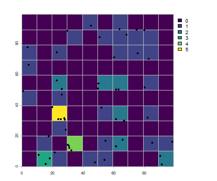
And a plot to inspect them.
plot(quads, border="gray", pax=list(las=1))
points(x, y, col="red", pch=20)
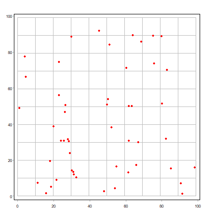
A standard question to ask is whether it is likely that this pattern was generated by random process. We can do this by comparing the observed frequencies with the theoretically expected frequencies. Note that in a coin toss the probability of success is 1/2; here the probability of success (the random chance that a point lands in quadrat is 1/(number of quadrats).
First count the number of points by quadrat (grid cell).
vxy <- vect(cbind(x,y))
vxy$v <- 1
p <- rasterize(vxy, r, "v", fun=length, background=0)
plot(p)
plot(quads, add=TRUE, border="gray")
points(x, y, pch=20)
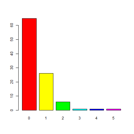
Get the frequency of the counts and make a barplot.
f <- freq(p)
f
##   layer value count
## 1     1     0    65
## 2     1     1    26
## 3     1     2     6
## 4     1     3     1
## 5     1     4     1
## 6     1     5     1
barplot(p)
To compare these observed values to the expected frequencies from the
binomial distribution we can use expected <- dbinom(n, size, prob).
In the book, this is P(k, n, x).
n <- 0:8
prob <- 1 / ncell(r)
size <- 50
expected <- dbinom(n, size, prob)
round(expected, 5)
## [1] 0.60501 0.30556 0.07562 0.01222 0.00145 0.00013 0.00001 0.00000 0.00000
plot(n, expected, cex=2, pch="x", col="blue")
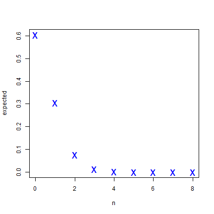
These numbers indicate that you would expect that most quadrats would have a point count of zero, a few would have 1 point, and very few more than that. Six or more points in a single cell is highly unlikely to happen if the data generating process in spatially random.
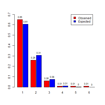
m <- rbind(f[,3]/100, expected[1:nrow(f)])
bp <- barplot(m, beside=T, names.arg =1:nrow(f), space=c(0.1, 0.5),
   ylim=c(0,0.7), col=c("red", "blue"))
text(bp, m, labels=round(m, 2), pos = 3, cex = .75)
legend(11, 0.7, c("Observed", "Expected"), fill=c("red", "blue"))
On page 106 it is discussed that the Poisson distribution can be a good approximation of the binomial distribution. Let’s get the expected values for the Poisson distribution. The intensity \(\lambda\) (lambda) is the number of points divided by the number of quadrats.
poisexp <- dpois(0:8, lambda=50/100)
poisexp
## [1] 6.065307e-01 3.032653e-01 7.581633e-02 1.263606e-02 1.579507e-03
## [6] 1.579507e-04 1.316256e-05 9.401827e-07 5.876142e-08
plot(expected, poisexp, cex=2)
abline(0,1)
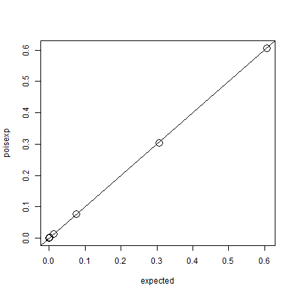
Pretty much the same, indeed.
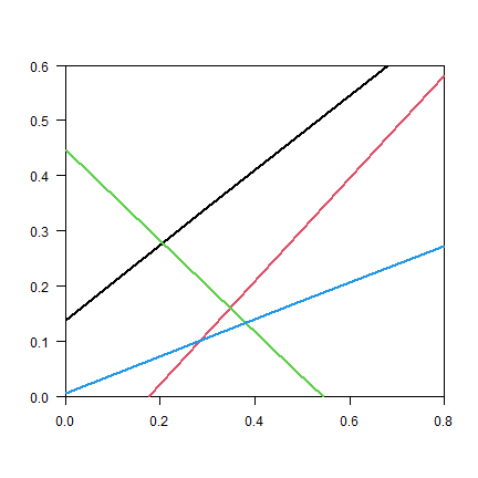
Random Lines
See pp 110-111. Here is a function that draws random lines through a rectangle. It first takes a random point within the rectangle, and a random angle. Then it uses basic trigonometry to find the line segments (where the line intersects with the rectangle). It returns the line length, or the coordinates of the intersection and random point, for plotting.
randomLineInRectangle <- function(xmn=0, xmx=0.8, ymn=0, ymx=0.6, retXY=FALSE) {
    x <- runif(1, xmn, xmx)
    y <- runif(1, ymn, ymx)
    angle <- runif(1, 0, 359.99999999)
    if (angle == 90) {
        # vertical line, tan is infinite
        if (retXY) {
            xy <- rbind(c(x, ymn), c(x, y), c(x, ymx))
            return(xy)
        }
        return(ymx - ymn)
    }
    tang <- tan(pi*angle/180)
    x1 <- max(xmn, min(xmx, x - y / tang))
    x2 <- max(xmn, min(xmx, x + (ymx-y) / tang))
    y1 <- max(ymn, min(ymx, y - (x-x1) * tang))
    y2 <- max(ymn, min(ymx, y + (x2-x) * tang))
    if (retXY) {
        xy <- rbind(c(x1, y1), c(x, y), c(x2, y2))
        return(xy)
    }
    sqrt((x2 - x1)^2 + (y2 - y1)^2)
}
We can test it:
randomLineInRectangle()
## [1] 0.4953701
randomLineInRectangle()
## [1] 0.4470846
set.seed(999)
plot(NA, xlim=c(0, 0.8), ylim=c(0, 0.6), xaxs="i", yaxs="i", xlab="", ylab="", las=1)
for (i in 1:4) {
    xy <- randomLineInRectangle(retXY=TRUE)
    lines(xy, lwd=2, col=i)
    #points(xy, cex=2, pch=20, col=i)
}
And plot the density function
r <- replicate(10000, randomLineInRectangle())
hist(r, breaks=seq(0,1,0.01), xlab="Line length", main="", freq=FALSE)
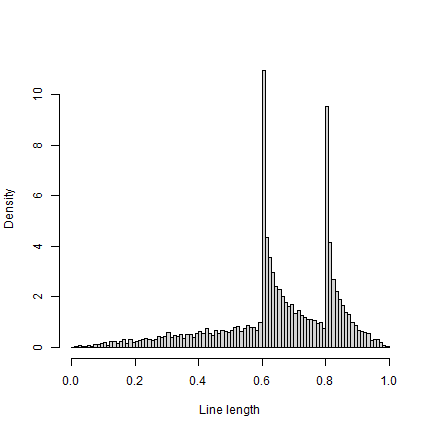
Note that the density function is similar to Fig 4.6, but not the same (e.g. for values near zero).
Sitting comfortably?
See the box on page 110-111. There are four seats on the table. Let’s number the seats 1, 2, 3, and 4. If two seats are occupied and the absolute difference between the seat numbers is 2, the customers sit straight across from each other. Otherwise, they sit across the corner from each other. What is the expected frequency of customers sitting straight across from each other? Let’s simulate.
set.seed(0)
x <- replicate(10000, abs(diff(sample(1:4, 2))))
sum(x==2) / length(x)
## [1] 0.3408
That is one third, as expected given that this represents two of the six ways you can sit.
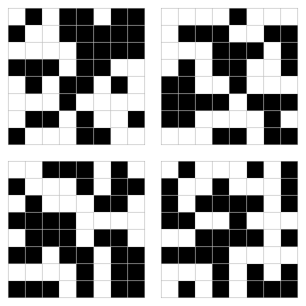
Random areas
Here is how you can create a function to create a “random chessboard” as described on page 114.
r <- rast(xmin=0, xmax=1, ymin=0, ymax=1, ncol=8, nrow=8)
p <- as.polygons(r)
chess <- function() {
    s <- sample(c(-1, 1), 64, replace=TRUE)
    values(r) <- s
    plot(r, col=c("black", "white"), legend=FALSE, axes=FALSE, mar=c(1,1,1,1))
    plot(p, add=T, border="gray")
}
And create four realizations:
set.seed(0)
par(mfrow=c(2,2))
for (i in 1:4) {
    chess()
}
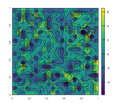
This is how you can create a random field (page 114/115)
r <- rast(xmin=0, xmax=1, ymin=0, ymax=1, ncol=20, nrow=20)
values(r) <- rnorm(ncell(r), 0, 2)
plot(r)
contour(r, add=T)
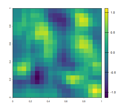
But a more realistic random field will have some spatial autocorrelation. We can create that with the focal function.
ra <- focal(r, w=matrix(1/9, nc=3, nr=3), na.rm=TRUE)
ra <- focal(ra, w=matrix(1/9, nc=3, nr=3), na.rm=TRUE)
plot(ra)
Questions
Use the examples provided above to write a script that follows the “thought exercise to fix ideas” on page 98 of OSU. Use a function to generate the random numbers. Use vectorization, that is, avoid using a for -loop or if statements
Use the example of the CSR point distribution to write a script that uses a normal distribution, rather than a random uniform distribution (also see box “different distributions”; on page 99 of OSU) and compares the generated pattern to the expected values.
How could you, conceptually, statistically test whether the real chessboard used in games is generated by an independent random process? What raster processing function might you use? (feel free to attempt to implement this, perhaps in simplified form)
Can you explain the odd distribution pattern of random line lengths inside a rectangle? It can helpful to write some code to separate different cases