Local statistics
Introduction
This handout accompanies Chapter 8 in O’Sullivan and Unwin (2010).
LISA
We compute some measures of local spatial autocorrelation.
First get the Auckland data.
if (!require("rspat")) remotes::install_github("rspatial/rspat")
library(rspat)
auck <- spat_data("auctb")
Now compute the spatial weights. You can try other ways
(e.g. relation="touches")
w <- relate(auck, relation="rook")
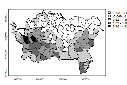
Compute the Getis Gi
Gi <- autocor(auck$TB, w, "Gi")
head(Gi)
## [1]  0.4241759  0.5623307  0.4047413  0.6819762 -1.3278352 -1.4086435
And make a map
grays <- rev(gray(seq(0,1,.2)))
auck$Gi <- Gi
plot(auck, "Gi", col=grays)
Now on to the Gi* by including the focal area in the computation.
#include "self"
diag(w) <- TRUE
auck$Gistar <- autocor(auck$TB, w, "Gi*")
plot(auck, "Gistar", main="Gi*", col=grays)
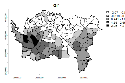
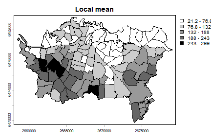
This looks very similar to the local average, which we compute below.
auck$loc_mean <- apply(w, 1, function(i) mean(auck$TB[i]))
plot(auck, "loc_mean", main="Local mean", col=grays)
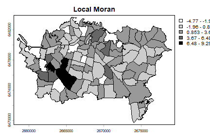
The local Moran Ii has not been implemented in terra, but we can
use spdep (a package that if focussed on these type of statistics
and on spatial regression).
library(spdep)
sfauck <- sf::st_as_sf(auck)
wr <- poly2nb(sfauck, row.names=sfauck$Id, queen=FALSE)
lstw <- nb2listw(wr, style="B")
auck$Ii <- localmoran(auck$TB, lstw)
## Warning: [[[<-,SpatVector] only using the first column
plot(auck, "Ii", main="Local Moran", col=grays)
In the above I followed the book by useing the raw count data. Howwever, it would be more approproate to use disease density instead. You can compute that like this:
auck$TBdens <- 10000 * auck$TB / expanse(auck)
The 10000 is just to avoid very small numbers.
Geographically weighted regression
Here is an example of GWR with California precipitation data.
cts <- spat_data("counties")
p <- spat_data("precipitation")
head(p)
## ID NAME LAT LONG ALT JAN FEB MAR APR MAY JUN JUL
## 1 ID741 DEATH VALLEY 36.47 -116.87 -59 7.4 9.5 7.5 3.4 1.7 1.0 3.7
## 2 ID743 THERMAL/FAA AIRPORT 33.63 -116.17 -34 9.2 6.9 7.9 1.8 1.6 0.4 1.9
## 3 ID744 BRAWLEY 2SW 32.96 -115.55 -31 11.3 8.3 7.6 2.0 0.8 0.1 1.9
## 4 ID753 IMPERIAL/FAA AIRPORT 32.83 -115.57 -18 10.6 7.0 6.1 2.5 0.2 0.0 2.4
## 5 ID754 NILAND 33.28 -115.51 -18 9.0 8.0 9.0 3.0 0.0 1.0 8.0
## 6 ID758 EL CENTRO/NAF 32.82 -115.67 -13 9.8 1.6 3.7 3.0 0.4 0.0 3.0
## AUG SEP OCT NOV DEC
## 1 2.8 4.3 2.2 4.7 3.9
## 2 3.4 5.3 2.0 6.3 5.5
## 3 9.2 6.5 5.0 4.8 9.7
## 4 2.6 8.3 5.4 7.7 7.3
## 5 9.0 7.0 8.0 7.0 9.0
## 6 10.8 0.2 0.0 3.3 1.4
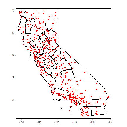
plot(cts)
points(p[,c("LONG", "LAT")], col="red", pch=20)
Compute annual average precipitation
p$pan <- rowSums(p[,6:17])
Global regression model
m <- lm(pan ~ ALT, data=p)
m
##
## Call:
## lm(formula = pan ~ ALT, data = p)
##
## Coefficients:
## (Intercept)          ALT
##      523.60         0.17
Create sf objects with a planar crs.
alb <- "+proj=aea +lat_1=34 +lat_2=40.5 +lat_0=0 +lon_0=-120 +x_0=0 +y_0=-4000000 +datum=WGS84"
sp <- vect(p, c("LONG", "LAT"), crs="+proj=longlat +datum=NAD83")
sp <- terra::project(sp, alb)
spsf <- sf::st_as_sf(sp)
vctst <- terra::project(cts, alb)
ctst <- sf::st_as_sf(vctst)
Get the optimal bandwidth
library( spgwr )
## Loading required package: sp
## NOTE: This package does not constitute approval of GWR
## as a method of spatial analysis; see example(gwr)
bw <- gwr.sel(pan ~ ALT, crds(sp), data=spsf)
## Bandwidth: 526221.2 CV score: 64886875
## Bandwidth: 850593.7 CV score: 74209068
## Bandwidth: 325748 CV score: 54001109
## Bandwidth: 201848.7 CV score: 44611208
## Bandwidth: 125274.7 CV score: 35746319
## Bandwidth: 77949.4 CV score: 29181740
## Bandwidth: 48700.75 CV score: 22737214
## Bandwidth: 30624.09 CV score: 17457187
## Bandwidth: 19452.1 CV score: 15163447
## Bandwidth: 12547.43 CV score: 19452244
## Bandwidth: 22792.76 CV score: 15513011
## Bandwidth: 17052.47 CV score: 15710047
## Bandwidth: 20218.98 CV score: 15167452
## Bandwidth: 19767.94 CV score: 15156926
## Bandwidth: 19790.02 CV score: 15156919
## Bandwidth: 19781.35 CV score: 15156915
## Bandwidth: 19781.45 CV score: 15156915
## Bandwidth: 19781.44 CV score: 15156915
## Bandwidth: 19781.44 CV score: 15156915
## Bandwidth: 19781.44 CV score: 15156915
## Bandwidth: 19781.44 CV score: 15156915
bw
## [1] 19781.44
Create a regular set of points to estimate parameters for.
r <- rast(vctst, res=10000)
r <- rasterize(vect(ctst), r)
newpts <- geom(as.points(r))[, c("x", "y")]
Run the gwr function
g <- gwr(pan ~ ALT, crds(sp), data=spsf, bandwidth=bw, fit.points=newpts[, 1:2])
g
## Call:
## gwr(formula = pan ~ ALT, data = spsf, coords = crds(sp), bandwidth = bw,
##     fit.points = newpts[, 1:2])
## Kernel function: gwr.Gauss
## Fixed bandwidth: 19781.44
## Fit points: 4090
## Summary of GWR coefficient estimates at fit points:
##                     Min.     1st Qu.      Median     3rd Qu.      Max.
## X.Intercept. -846.296586   77.986455  328.578859  729.603430 3452.2039
## ALT            -3.961769    0.034145    0.201568    0.418717    4.6023
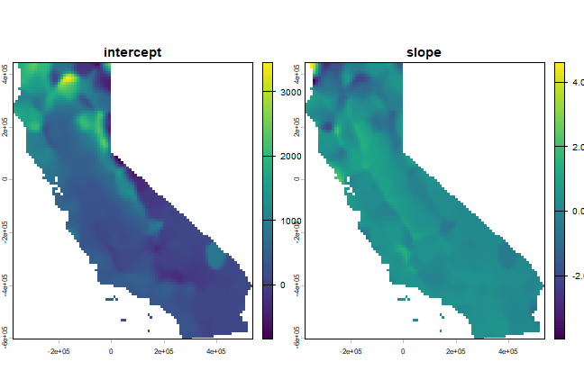
Link the results back to the raster.
slope <- intercept <- r
slope[!is.na(slope)] <- g$SDF$ALT
intercept[!is.na(intercept)] <- g$SDF$"(Intercept)"
s <- c(intercept, slope)
names(s) <- c("intercept", "slope")
plot(s)
See this page for a more detailed example of geographically weighted regression.