Environmental data
Raster data
In species distribution modeling, predictor variables are typically
organized as raster (grid) type files. Each predictor should be a
‘raster’ representing a variable of interest. Variables can include
climatic, soil, terrain, vegetation, land use, and other variables.
These data are typically stored in files in some kind of GIS format.
Almost all relevant formats can be used (including ESRI grid, geoTiff,
netCDF, IDRISI). Avoid ASCII files if you can, as they tend to
considerably slow down processing speed. For any particular study the
layers should all have the same spatial extent, resolution, origin, and
projection. If necessary, use functions like crop, extend,
aggregate, resample, and projectRaster from the raster
package. See the Introduction to spatial data
manipulation for more information
about function you can use to prepare your predictor variable data. See
the help files and the vignette of the raster package for more info on
how to do this.
The set of predictor variables (rasters) can be used to make a
RasterStack, which is a collection of `RasterLayer’ objects (see
the Spatial Data tutorial for more
info.
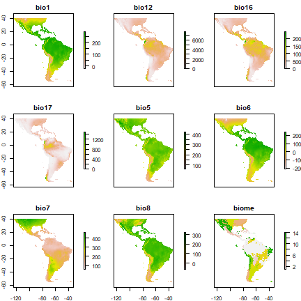
Here we make a list of files that are installed with the dismo package and then create a rasterStack from these, show the names of each layer, and finally plot them all.
First get the folder with our files. In this example it is the (“ex”) directory of the dismo package. You do not need such a complex statement to get your own files (you just type the string).
path <- file.path(system.file(package="dismo"), 'ex')
Now get the names of all the files with extension “.grd” in this folder.
The $ sign indicates that the files must end with the characters
‘grd’. By using full.names=TRUE, the full path names are retunred.
library(dismo)
files <- list.files(path, pattern='grd$', full.names=TRUE )
files
## [1] "C:/soft/R/R-devel/library/dismo/ex/bio1.grd"
## [2] "C:/soft/R/R-devel/library/dismo/ex/bio12.grd"
## [3] "C:/soft/R/R-devel/library/dismo/ex/bio16.grd"
## [4] "C:/soft/R/R-devel/library/dismo/ex/bio17.grd"
## [5] "C:/soft/R/R-devel/library/dismo/ex/bio5.grd"
## [6] "C:/soft/R/R-devel/library/dismo/ex/bio6.grd"
## [7] "C:/soft/R/R-devel/library/dismo/ex/bio7.grd"
## [8] "C:/soft/R/R-devel/library/dismo/ex/bio8.grd"
## [9] "C:/soft/R/R-devel/library/dismo/ex/biome.grd"
Now create a RasterStack of predictor variables.
predictors <- stack(files)
predictors
## class      : RasterStack
## dimensions : 192, 186, 35712, 9  (nrow, ncol, ncell, nlayers)
## resolution : 0.5, 0.5  (x, y)
## extent     : -125, -32, -56, 40  (xmin, xmax, ymin, ymax)
## crs        : +proj=longlat +datum=WGS84 +no_defs
## names      : bio1, bio12, bio16, bio17, bio5, bio6, bio7, bio8, biome
## min values :  -23,     0,     0,     0,   61, -212,   60,  -66,     1
## max values :  289,  7682,  2458,  1496,  422,  242,  461,  323,    14
names(predictors)
## [1] "bio1"  "bio12" "bio16" "bio17" "bio5"  "bio6"  "bio7"  "bio8"  "biome"
plot(predictors)
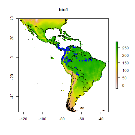
We can also make a plot of a single layer in a RasterStack, and plot some additional data on top of it. First get the world boundaries and the bradypus data:
library(maptools)
data(wrld_simpl)
file <- paste(system.file(package="dismo"), "/ex/bradypus.csv", sep="")
bradypus <- read.table(file,  header=TRUE,  sep=',')
# we do not need the first column
bradypus  <- bradypus[,-1]
And now plot:
# first layer of the RasterStack
plot(predictors, 1)
# note the "add=TRUE" argument with plot
plot(wrld_simpl, add=TRUE)
# with the points function, "add" is implicit
points(bradypus, col='blue')
The example above uses data representing ‘bioclimatic variables’ from
the WorldClim database (Hijmans et al.,
2004) and ‘terrestrial
biome’ data
from the WWF (Olsen et al., 2001). You can go to these websites if you
want higher resolution data. You can also use the getData function
from the raster package to download WorldClim climate data.
Predictor variable selection can be important, particularly if the
objective of a study is explanation. See, e.g., Austin and Smith (1987),
Austin (2002), Mellert et al., (2011). The early applications of
species modeling tended to focus on explanation (Elith and Leathwick
2009). Nowadays, the objective of SDM tends to be prediction. For
prediction within the same geographic area, variable selection might
arguably be relatively less important, but for many prediction tasks
(e.g. to new times or places, see below) variable selection is
critically important. In all cases it is important to use variables that
are relevant to the ecology of the species (rather than with the first
dataset that can be found on the web!). In some cases it can be useful
to develop new, more ecologically relevant, predictor variables from
existing data. For example, one could use land cover data and the
focal function in the raster package to create a new variable
that indicates how much forest area is available within x km of a grid
cell, for a species that might have a home range of x.
Extracting values from rasters
We now have a set of predictor variables (rasters) and occurrence
points. The next step is to extract the values of the predictors at the
locations of the points. (This step can be skipped for the modeling
methods that are implemented in the dismo package). This is a very
straightforward thing to do using the ‘extract’ function from the raster
package. In the example below we use that function first for the
Bradypus occurrence points, then for 500 random background points.
We combine these into a single data.frame in which the first column
(variable ‘pb’) indicates whether this is a presence or a background
point. ‘biome’ is categorical variable (called a ‘factor’ in R) and it
is important to explicitly define it that way, so that it won’t be
treated like any other numerical variable.
presvals <- extract(predictors, bradypus)
# setting random seed to always create the same
# random set of points for this example
set.seed(0)
backgr <- randomPoints(predictors, 500)
absvals <- extract(predictors, backgr)
pb <- c(rep(1, nrow(presvals)), rep(0, nrow(absvals)))
sdmdata <- data.frame(cbind(pb, rbind(presvals, absvals)))
sdmdata[,'biome'] = as.factor(sdmdata[,'biome'])
head(sdmdata)
##   pb bio1 bio12 bio16 bio17 bio5 bio6 bio7 bio8 biome
## 1  1  263  1639   724    62  338  191  147  261     1
## 2  1  263  1639   724    62  338  191  147  261     1
## 3  1  253  3624  1547   373  329  150  179  271     1
## 4  1  243  1693   775   186  318  150  168  264     1
## 5  1  243  1693   775   186  318  150  168  264     1
## 6  1  252  2501  1081   280  326  154  172  270     1
tail(sdmdata)
##     pb bio1 bio12 bio16 bio17 bio5 bio6 bio7 bio8 biome
## 611  0  265  1622   749    66  344  184  160  266     1
## 612  0  241  1648   475   354  294  183  112  229     1
## 613  0  154   731   250    80  319   18  301  198     8
## 614  0  169  1195   316   273  293   69  224  122     7
## 615  0  247  2965  1173   327  314  168  146  253     1
## 616  0  117   495   231    36  336  -96  432  216     8
summary(sdmdata)
##        pb              bio1           bio12            bio16
##  Min.   :0.0000   Min.   : 16.0   Min.   :   0.0   Min.   :   0.0
##  1st Qu.:0.0000   1st Qu.:176.8   1st Qu.: 821.5   1st Qu.: 341.8
##  Median :0.0000   Median :242.0   Median :1497.0   Median : 645.5
##  Mean   :0.1883   Mean   :213.9   Mean   :1629.5   Mean   : 656.4
##  3rd Qu.:0.0000   3rd Qu.:261.0   3rd Qu.:2266.8   3rd Qu.: 917.0
##  Max.   :1.0000   Max.   :286.0   Max.   :7682.0   Max.   :2458.0
##
##      bio17             bio5            bio6             bio7
##  Min.   :   0.0   Min.   : 88.0   Min.   :-167.0   Min.   : 68.0
##  1st Qu.:  42.0   1st Qu.:303.0   1st Qu.:  45.0   1st Qu.:118.8
##  Median : 110.0   Median :320.0   Median : 151.0   Median :160.0
##  Mean   : 169.2   Mean   :309.3   Mean   : 119.3   Mean   :190.0
##  3rd Qu.: 240.5   3rd Qu.:333.0   3rd Qu.: 202.2   3rd Qu.:247.0
##  Max.   :1496.0   Max.   :410.0   Max.   : 232.0   Max.   :440.0
##
##       bio8           biome
##  Min.   :-20.0   1      :299
##  1st Qu.:215.0   7      : 65
##  Median :250.0   8      : 61
##  Mean   :225.1   13     : 51
##  3rd Qu.:262.0   2      : 49
##  Max.   :323.0   4      : 33
##                  (Other): 58
There are alternative approaches possible here. For example, one could extract multiple points in a radius as a potential means for dealing with mismatch between location accuracy and grid cell size. If one would make 10 datasets that represent 10 equally valid “samples” of the environment in that radius, that could be then used to fit 10 models and explore the effect of uncertainty in location.
To visually investigate colinearity in the environmental data (at the presence and background points) you can use a pairs plot. See Dormann et al. (2013) for a discussion of methods to remove colinearity.
pairs(sdmdata[,2:5], cex=0.1)
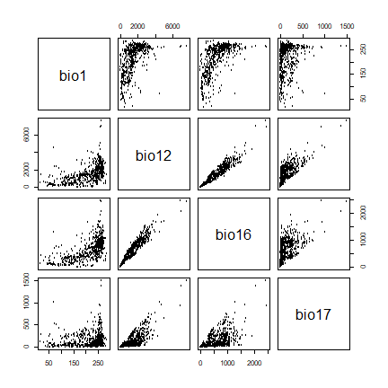
A pairs plot of the values of the climate data at the Bradypus occurrence sites.
To use the sdmdata and presvals in the next chapter, we save it
to disk.
saveRDS(sdmdata, "sdm.Rds")
saveRDS(presvals, "pvals.Rds")