Model fitting, prediction, and evaluation
Model fitting
Model fitting is technically quite similar across the modeling methods
that exist in R. Most methods take a formula identifying the
dependent and independent variables, accompanied with a data.frame
that holds these variables. Details on specific methods are provided
further down on this document, in part III.
A simple formula could look like: y ~ x1 + x2 + x3, i.e., y is a
function of x1, x2, and x3. Another example is y ~ ., which means
that y is a function of all other variables in the data.frame
provided to the function. See help('formula') for more details about
the formula syntax. In the example below, the function glm is used
to fit generalized linear models. glm returns a model object.
Note that in the examples below, we are using the data.frame ‘sdmdata’
again. First read sdmdata from disk (we saved it at the end of the
previous chapter).
library(dismo)
sdmdata <- readRDS("sdm.Rds")
presvals <- readRDS("pvals.Rds")
m1 <- glm(pb ~ bio1 + bio5 + bio12, data=sdmdata)
class(m1)
## [1] "glm" "lm"
summary(m1)
##
## Call:
## glm(formula = pb ~ bio1 + bio5 + bio12, data = sdmdata)
##
## Deviance Residuals:
##      Min        1Q    Median        3Q       Max
## -0.95534  -0.23380  -0.09987   0.07831   0.88796
##
## Coefficients:
##               Estimate Std. Error t value Pr(>|t|)
## (Intercept)  1.550e-01  1.093e-01   1.418 0.156593
## bio1         1.621e-03  3.960e-04   4.093 4.84e-05 ***
## bio5        -1.614e-03  4.725e-04  -3.417 0.000676 ***
## bio12        1.140e-04  1.676e-05   6.806 2.39e-11 ***
## ---
## Signif. codes:  0 '***' 0.001 '**' 0.01 '*' 0.05 '.' 0.1 ' ' 1
##
## (Dispersion parameter for gaussian family taken to be 0.1220413)
##
##     Null deviance: 94.156  on 615  degrees of freedom
## Residual deviance: 74.689  on 612  degrees of freedom
## AIC: 458.43
##
## Number of Fisher Scoring iterations: 2
m2 = glm(pb ~ ., data=sdmdata)
m2
##
## Call:  glm(formula = pb ~ ., data = sdmdata)
##
## Coefficients:
## (Intercept)         bio1        bio12        bio16        bio17         bio5
##   0.2644272   -0.0020029    0.0004336   -0.0006207   -0.0007843    0.0035996
##        bio6         bio7         bio8       biome2       biome3       biome4
##  -0.0025153   -0.0041593    0.0008508   -0.0899869   -0.1262125   -0.0699228
##      biome5       biome7       biome8       biome9      biome10      biome11
##  -0.0136612   -0.1993102    0.0057666    0.0465949    0.0055868   -0.2705639
##     biome12      biome13      biome14
##  -0.0450194    0.0839402   -0.1689054
##
## Degrees of Freedom: 615 Total (i.e. Null);  595 Residual
## Null Deviance:       94.16
## Residual Deviance: 69.17     AIC: 445.1
Models that are implemented in dismo do not use a formula (and most models only take presence points). Bioclim is an example. It only uses presence data, so we use ‘presvals’ instead of ‘sdmdata’.
bc <- bioclim(presvals[,c('bio1', 'bio5', 'bio12')])
class(bc)
## [1] "Bioclim"
## attr(,"package")
## [1] "dismo"
bc
## class : Bioclim
##
## variables: bio1 bio5 bio12
##
##
## presence points: 116
## bio1 bio5 bio12
## 1 263 338 1639
## 2 263 338 1639
## 3 253 329 3624
## 4 243 318 1693
## 5 243 318 1693
## 6 252 326 2501
## 7 240 317 1214
## 8 275 335 2259
## 9 271 327 2212
## 10 274 329 2233
## (... ... ...)
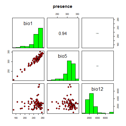
pairs(bc)
Model prediction
Different modeling methods return different type of ‘model’ objects
(typically they have the same name as the modeling method used). All of
these ‘model’ objects, irrespective of their exact class, can be used to
with the predict function to make predictions for any combination of
values of the independent variables. This is illustrated in the example
below where we make predictions with the glm model object ‘m1’ and for
bioclim model ‘bc’, for three records with values for variables bio1,
bio5 and bio12 (the variables used in the example above to create the
model objects).
bio1 = c(40, 150, 200)
bio5 = c(60, 115, 290)
bio12 = c(600, 1600, 1700)
pd = data.frame(cbind(bio1, bio5, bio12))
pd
##   bio1 bio5 bio12
## 1   40   60   600
## 2  150  115  1600
## 3  200  290  1700
predict(m1, pd)
##         1         2         3
## 0.1914136 0.3949569 0.2048905
predict(bc, pd)
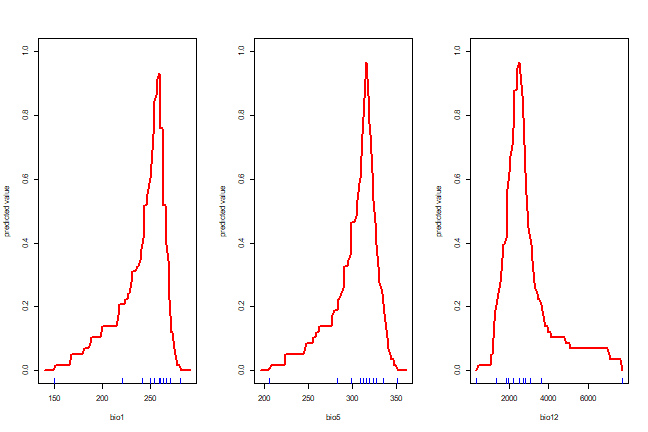
Making such predictions for a few environments can be very useful to
explore and understand model predictions. For example it used in the
response function that creates response plots for each variable,
with the other variables at their median value.
response(bc)
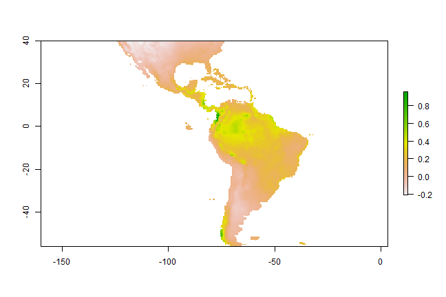
In most cases, howver, the purpose is SDM is to create a map of suitability scores. We can do that by providing the predict function with a Raster* object and a model object. As long as the variable names in the model object are available as layers (layerNames) in the Raster* object.
predictors <- stack(list.files(file.path(system.file(package="dismo"), 'ex'), pattern='grd$', full.names=TRUE ))
names(predictors)
## [1] "bio1"  "bio12" "bio16" "bio17" "bio5"  "bio6"  "bio7"  "bio8"  "biome"
p <- predict(predictors, m1)
plot(p)
Model evaluation
It is much easier to create a model and make a prediction than to assess how good the model is, and whether it is can be used for a specific purpose. Most model types have different measures that can help to assess how good the model fits the data. It is worth becoming familiar with these and understanding their role, because they help you to assess whether there is anything substantially wrong with your model. Most statistics or machine learning texts will provide some details. For instance, for a GLM one can look at how much deviance is explained, whether there are patterns in the residuals, whether there are points with high leverage and so on. However, since many models are to be used for prediction, much evaluation is focused on how well the model predicts to points not used in model training (see following section on data partitioning). Before we start to give some examples of statistics used for this evaluation, it is worth considering what else can be done to evaluate a model. Useful questions include:
Does the model seem sensible, ecologically?
Do the fitted functions (the shapes of the modeled relationships) make sense?
Do the predictions seem reasonable? (map them, and think about them)?
Are there any spatial patterns in model residuals? (see Leathwick and Whitehead 2001 for an interesting example)
Most modelers rely on cross-validation. This consists of creating a model with one ‘training’ data set, and testing it with another data set of known occurrences. Typically, training and testing data are created through random sampling (without replacement) from a single data set. Only in a few cases, e.g. Elith et al., 2006, training and test data are from different sources and pre-defined.
Different measures can be used to evaluate the quality of a prediction (Fielding and Bell, 1997, Liu et al., 2011; and Potts and Elith (2006) for abundance data), perhaps depending on the goal of the study. Many measures for evaluating models based on presence-absence or presence-only data are ‘threshold dependent’. That means that a threshold must be set first (e.g., 0.5, though 0.5 is rarely a sensible choice – e.g. see Lui et al. 2005). Predicted values above that threshold indicate a prediction of ‘presence’, and values below the threshold indicate ‘absence’. Some measures emphasize the weight of false absences; others give more weight to false presences.
Much used statistics that are threshold independent are the correlation coefficient and the Area Under the Receiver Operator Curve (AUROC, generally further abbreviated to AUC). AUC is a measure of rank-correlation. In unbiased data, a high AUC indicates that sites with high predicted suitability values tend to be areas of known presence and locations with lower model prediction values tend to be areas where the species is not known to be present (absent or a random point). An AUC score of 0.5 means that the model is as good as a random guess. See Phillips et al. (2006) for a discussion on the use of AUC in the context of presence-only rather than presence/absence data.
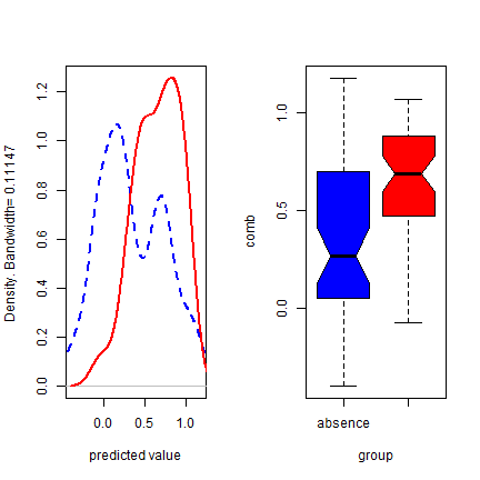
Here we illustrate the computation of the correlation coefficient and
AUC with two random variables. p (presence) has higher values, and
represents the predicted value for 50 known cases (locations) where the
species is present, and a (absence) has lower values, and represents
the predicted value for 50 known cases (locations) where the species is
absent.
p <- rnorm(50, mean=0.7, sd=0.3)
a <- rnorm(50, mean=0.4, sd=0.4)
par(mfrow=c(1, 2))
plot(sort(p), col='red', pch=21)
points(sort(a), col='blue', pch=24)
legend(1, 0.95 * max(a,p), c('presence', 'absence'),
          pch=c(21,24), col=c('red', 'blue'))
comb <- c(p,a)
group <- c(rep('presence', length(p)), rep('absence', length(a)))
boxplot(comb~group, col=c('blue', 'red'))
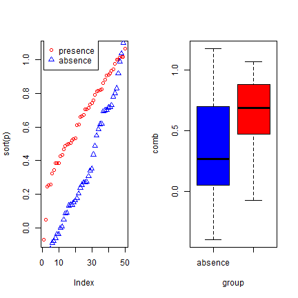
We created two variables with random normally distributed values, but with different mean and standard deviation. The two variables clearly have different distributions, and the values for ‘presence’ tend to be higher than for ‘absence’. Here is how you can compute the correlation coefficient and the AUC:
group = c(rep(1, length(p)), rep(0, length(a)))
cor.test(comb, group)$estimate
##       cor
## 0.4151511
mv <- wilcox.test(p,a)
auc <- as.numeric(mv$statistic) / (length(p) * length(a))
auc
## [1] 0.7344
Below we show how you can compute these, and other statistics more
conveniently, with the evaluate function in the dismo package. See
?evaluate for info on additional evaluation measures that are
available. ROC/AUC can also be computed with the ROCR package.
e <- evaluate(p=p, a=a)
class(e)
## [1] "ModelEvaluation"
## attr(,"package")
## [1] "dismo"
e
## class          : ModelEvaluation
## n presences    : 50
## n absences     : 50
## AUC            : 0.7344
## cor            : 0.4151511
## max TPR+TNR at : 0.3219399
par(mfrow=c(1, 2))
density(e)
boxplot(e, col=c('blue', 'red'))
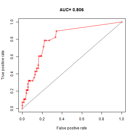
Back to some real data, presence-only in this case. We’ll divide the data in two random sets, one for training a Bioclim model, and one for evaluating the model.
samp <- sample(nrow(sdmdata), round(0.75 * nrow(sdmdata)))
traindata <- sdmdata[samp,]
traindata <- traindata[traindata[,1] == 1, 2:9]
testdata <- sdmdata[-samp,]
bc <- bioclim(traindata)
e <- evaluate(testdata[testdata==1,], testdata[testdata==0,], bc)
e
## class          : ModelEvaluation
## n presences    : 28
## n absences     : 126
## AUC            : 0.805839
## cor            : 0.4028775
## max TPR+TNR at : 0.09080909
plot(e, 'ROC')
In real projects, you would want to use k-fold data partitioning
instead of a single random sample. The dismo function kfold
facilitates that type of data partitioning. It creates a vector that
assigns each row in the data matrix to a a group (between 1 to k).
Let’s first create presence and background data.
pres <- sdmdata[sdmdata[,1] == 1, 2:9]
back <- sdmdata[sdmdata[,1] == 0, 2:9]
The background data will only be used for model testing and does not need to be partitioned. We now partition the data into 5 groups.
k <- 5
group <- kfold(pres, k)
group[1:10]
##  [1] 5 2 3 1 5 1 1 1 3 3
unique(group)
## [1] 5 2 3 1 4
Now we can fit and test our model five times. In each run, the records corresponding to one of the five groups is only used to evaluate the model, while the other four groups are only used to fit the model. The results are stored in a list called ‘e’.
e <- list()
for (i in 1:k) {
    train <- pres[group != i,]
    test <- pres[group == i,]
    bc <- bioclim(train)
    e[[i]] <- evaluate(p=test, a=back, bc)
}
We can extract several things from the objects in ‘e’, but let’s restrict ourselves to the AUC values and the “maximum of the sum of the sensitivity (true positive rate) and specificity (true negative rate)” threshold “spec_sens” (this is sometimes uses as a threshold for setting cells to presence or absence).
auc <- sapply(e, function(x){x@auc})
auc
## [1] 0.7739565 0.8291739 0.7931250 0.7588696 0.7660435
mean(auc)
## [1] 0.7842337
sapply( e, function(x){ threshold(x)['spec_sens'] } )
## $spec_sens
## [1] 0.01065269
##
## $spec_sens
## [1] 0.07516882
##
## $spec_sens
## [1] 0.1085957
##
## $spec_sens
## [1] 0.02140538
##
## $spec_sens
## [1] 0.06441613
The use of AUC in evaluating SDMs has been criticized (Lobo et al. 2008, Jiménez-Valverde 2011). A particularly sticky problem is that the values of AUC vary with the spatial extent used to select background points. Generally, the larger that extent, the higher the AUC value. Therefore, AUC values are generally biased and cannot be directly compared. Hijmans (2012) suggests that one could remove “spatial sorting bias” (the difference between the distance from testing-presence to training-presence and the distance from testing-absence to training-presence points) through “point-wise distance sampling”.
file <- file.path(system.file(package="dismo"), "ex/bradypus.csv")
bradypus <- read.table(file,  header=TRUE,  sep=',')
bradypus <- bradypus[,-1]
presvals <- extract(predictors, bradypus)
set.seed(0)
backgr <- randomPoints(predictors, 500)
nr <- nrow(bradypus)
s <- sample(nr, 0.25 * nr)
pres_train <- bradypus[-s, ]
pres_test <- bradypus[s, ]
nr <- nrow(backgr)
set.seed(9)
s <- sample(nr, 0.25 * nr)
back_train <- backgr[-s, ]
back_test <- backgr[s, ]
sb <- ssb(pres_test, back_test, pres_train)
sb[,1] / sb[,2]
##         p
## 0.1000638
sb[,1] / sb[,2] is an indicator of spatial sorting bias (SSB). If
there is no SSB this value should be 1, in these data it is close to
zero, indicating that SSB is very strong. Let’s create a subsample in
which SSB is removed.
i <- pwdSample(pres_test, back_test, pres_train, n=1, tr=0.1)
pres_test_pwd <- pres_test[!is.na(i[,1]), ]
back_test_pwd <- back_test[na.omit(as.vector(i)), ]
sb2 <- ssb(pres_test_pwd, back_test_pwd, pres_train)
sb2[1]/ sb2[2]
## [1] 1.004106
Spatial sorting bias is much reduced now; notice how the AUC dropped!
bc <- bioclim(predictors, pres_train)
evaluate(bc, p=pres_test, a=back_test, x=predictors)
## class          : ModelEvaluation
## n presences    : 29
## n absences     : 125
## AUC            : 0.757931
## cor            : 0.2777298
## max TPR+TNR at : 0.03438276
evaluate(bc, p=pres_test_pwd, a=back_test_pwd, x=predictors)
## class          : ModelEvaluation
## n presences    : 19
## n absences     : 19
## AUC            : 0.5914127
## cor            : 0.1487003
## max TPR+TNR at : 0.09185402