Geographic Null models
The ‘geographic Null models’ described here are not commonly used in species distribution modeling. They use the geographic location of known occurrences, and do not rely on the values of predictor variables at these locations. We are exploring their use in comparing and contrasting them with the other approaches (Bahn and McGill, 2007); in model evaluation as as null-models (Hijmans 2012); to sample background points; and generally to help think about the duality between geographic and environmental space (Collwel and Rangel, 2009). Below we show examples of these different types of models.
Geographic Distance
Simple model based on the assumption that the closer to a know presence point, the more likely it is to find the species.
Recreate our data.
library(dismo)
predictors <- stack(list.files(path=file.path(system.file(package="dismo"), 'ex'), pattern='grd$', full.names=TRUE ))
ext <- extent(-90, -32, -33, 23)
bradypus <- read.csv(file.path(system.file(package="dismo"), "ex/bradypus.csv"))[,-1]
set.seed(0)
group <- kfold(bradypus, 5)
pres_train <- bradypus[group != 1, ]
pres_test <- bradypus[group == 1, ]
set.seed(0)
backgr <- randomPoints(predictors, 500)
set.seed(9)
nr <- nrow(backgr)
s <- sample(nr, 0.25 * nr)
back_train <- backgr[-s, ]
back_test <- backgr[s, ]
set.seed(10)
pred_nf <- dropLayer(predictors, 'biome')
backg <- randomPoints(pred_nf, n=1000, ext=ext, extf = 1.25)
colnames(backg) = c('lon', 'lat')
group <- kfold(backg, 5)
backg_train <- backg[group != 1, ]
backg_test <- backg[group == 1, ]
library(maptools)
data(wrld_simpl)
First create a mask to predict to, and to use as a mask to only predict to land areas.
seamask <- crop(predictors[[1]], ext)
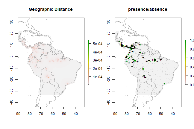
distm <- geoDist(pres_train, lonlat=TRUE)
ds <- predict(seamask, distm, mask=TRUE)
e <- evaluate(distm, p=pres_test, a=backg_test)
e
## class : ModelEvaluation
## n presences : 23
## n absences : 200
## AUC : 0.9015217
## cor : 0.4564334
## max TPR+TNR at : 2.217e-05
And the plots.
par(mfrow=c(1,2))
plot(ds, main='Geographic Distance')
plot(wrld_simpl, add=TRUE, border='dark grey')
tr <- threshold(e, 'spec_sens')
plot(ds > tr, main='presence/absence')
plot(wrld_simpl, add=TRUE, border='dark grey')
points(pres_train, pch='+')
points(backg_train, pch='-', cex=0.25)
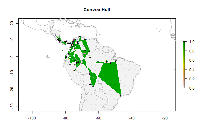
Convex hulls
This model draws a convex hull around all ‘presence’ points.
hull <- convHull(pres_train, lonlat=TRUE)
e <- evaluate(hull, p=pres_test, a=backg_test)
e
## class          : ModelEvaluation
## n presences    : 23
## n absences     : 200
## AUC            : 0.5646739
## cor            : 0.1006176
## max TPR+TNR at : 0.9999
h <- predict(seamask, hull, mask=TRUE)
plot(h, main='Convex Hull')
plot(wrld_simpl, add=TRUE, border='dark grey')
points(pres_train, pch='+')
points(backg_train, pch='-', cex=0.25)
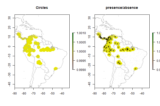
Circles
This model draws circles around all ‘presence’ points.
circ <- circles(pres_train, lonlat=TRUE)
pc <- predict(seamask, circ, mask=TRUE)
e <- evaluate(circ, p=pres_test, a=backg_test)
e
## class          : ModelEvaluation
## n presences    : 23
## n absences     : 200
## AUC            : 0.8297826
## cor            : 0.447742
## max TPR+TNR at : 0.9999
par(mfrow=c(1,2))
plot(pc, main='Circles')
plot(wrld_simpl, add=TRUE, border='dark grey')
tr <- threshold(e, 'spec_sens')
plot(pc > tr, main='presence/absence')
plot(wrld_simpl, add=TRUE, border='dark grey')
points(pres_train, pch='+')
points(backg_train, pch='-', cex=0.25)
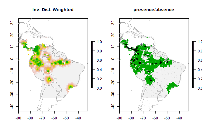
Presence/absence
Spatial-only models for presence/background (or absence) data are also
available through functions geoIDW, voronoiHull, and general
geostatistical methods such as indicator kriging (available in the
“gstat” package).
idwm <- geoIDW(p=pres_train, a=data.frame(back_train))
e <- evaluate(idwm, p=pres_test, a=backg_test)
e
## class          : ModelEvaluation
## n presences    : 23
## n absences     : 200
## AUC            : 0.8702174
## cor            : 0.4548002
## max TPR+TNR at : 0.03483593
iw <- predict(seamask, idwm, mask=TRUE)
par(mfrow=c(1,2))
plot(iw, main='Inv. Dist. Weighted')
plot(wrld_simpl, add=TRUE, border='dark grey')
tr <- threshold(e, 'spec_sens')
pa <- mask(iw > tr, seamask)
plot(pa, main='presence/absence')
plot(wrld_simpl, add=TRUE, border='dark grey')
points(pres_train, pch='+')
points(backg_train, pch='-', cex=0.25)
# take a smallish sample of the background training data
va <- data.frame(back_train[sample(nrow(back_train), 100), ])
vorm <- voronoiHull(p=pres_train, a=va)
e <- evaluate(vorm, p=pres_test, a=backg_test)
e
## class : ModelEvaluation
## n presences : 23
## n absences : 200
## AUC : 0.49
## cor : -0.04326367
## max TPR+TNR at : 0.9999
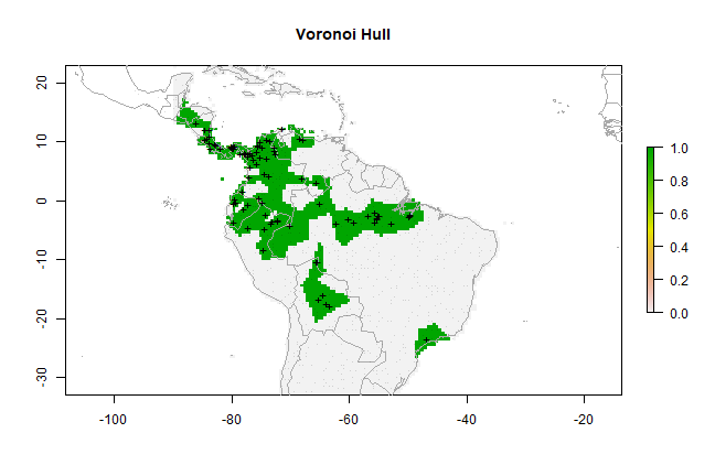
vo <- predict(seamask, vorm, mask=T)
plot(vo, main='Voronoi Hull')
plot(wrld_simpl, add=TRUE, border='dark grey')
points(pres_train, pch='+')
points(backg_train, pch='-', cex=0.25)