Appendix: Boosted regression trees for ecological modeling
Jane Elith and John Leathwick
Introduction
This is a brief tutorial to accompany a set of functions that we have written to facilitate fitting BRT (boosted regression tree) models in R. This tutorial is a modified version of the tutorial accompanying Elith, Leathwick and Hastie’s article in Journal of Animal Ecology. It has been adjusted to match the implementation of these functions in the ‘dismo’ package. The gbm* functions in the dismo package extend functions in the ‘gbm’ package by Greg Ridgeway. The goal of our functions is to make the functions in the ‘gbm’ package easier to apply to ecological data, and to enhance interpretation.
The tutorial is aimed at helping you to learn the mechanics of how to use the functions and to develop a BRT model in R. It does not explain what a BRT model is - for that, see the references at the end of the tutorial, and the documentation of the gbm package. For an example application with similar data as in this tutorial, see Elith et al., 2008.
The gbm functions in ‘dismo’ are as follows:
gbm.step- Fits a gbm model to one or more response variables, using cross-validation to estimate the optimal number of trees. This requires use of the utility functions roc, calibration and calc.deviance.gbm.fixed,gbm.holdout- Alternative functions for fitting gbm models, implementing options provided in the gbm package.gbm.simplify- Code to perform backwards elimination of variables, to drop those that give no evidence of improving predictive performance.gbm.plot- Plots the partial dependence of the response on one or more predictors.gbm.plot.fits- Plots the fitted values from a gbm object returned by any of the model fitting options. This can give a more reliable guide to the shape of the fitted surface than can be obtained from the individual functions, particularly when predictor variables are correlated and/or samples are unevenly distributed in environmental space.gbm.interactions- Tests whether interactions have been detected and modelled, and reports the relative strength of these. Results can be visualised with gbm.perspec
Example data
Two sets of presence/absence data for Anguilla australis (Angaus) are available. One for model training (building) and one for model testing (evaluation). In the example below we load the training data. Presence (1) and absence (0) is recorded in column 2. The environmental variables are in columns 3 to 14. This is the same data as used in Elith, Leathwick and Hastie (2008).
library(dismo)
data(Anguilla_train)
head(Anguilla_train)
##   Site Angaus SegSumT SegTSeas SegLowFlow DSDist DSMaxSlope USAvgT USRainDays
## 1    1      0    16.0    -0.10      1.036  50.20       0.57   0.09      2.470
## 2    2      1    18.7     1.51      1.003 132.53       1.15   0.20      1.153
## 3    3      0    18.3     0.37      1.001 107.44       0.57   0.49      0.847
## 4    4      0    16.7    -3.80      1.000 166.82       1.72   0.90      0.210
## 5    5      1    17.2     0.33      1.005   3.95       1.15  -1.20      1.980
## 6    6      0    15.1     1.83      1.015  11.17       1.72  -0.20      3.300
##   USSlope USNative DSDam   Method LocSed
## 1     9.8     0.81     0 electric    4.8
## 2     8.3     0.34     0 electric    2.0
## 3     0.4     0.00     0      spo    1.0
## 4     0.4     0.22     1 electric    4.0
## 5    21.9     0.96     0 electric    4.7
## 6    25.7     1.00     0 electric    4.5
Fitting a model
To fit a gbm model, you need to decide what settings to use the article
associated with this tutorial gives you information on what to use as
rules of thumb. These data have 1000 sites, comprising 202 presence
records for the short-finned eel (the command sum(model.data$Angaus)
will give you the total number of presences). As a first guess you could
decide:
There are enough data to model interactions of reasonable complexity
A lr of about 0.01 could be a reasonable starting point.
To below example shows how to use our function that steps forward and identifies the optimal number of trees (nt).
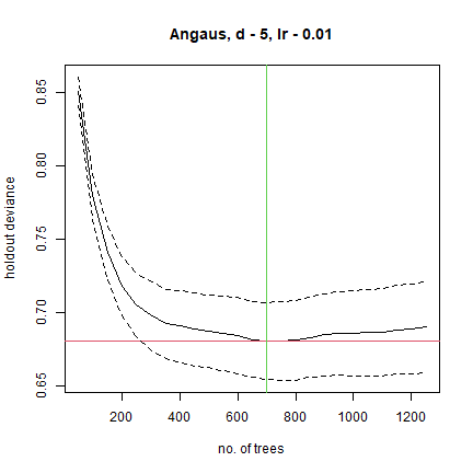
angaus.tc5.lr01 <- gbm.step(data=Anguilla_train, gbm.x = 3:13, gbm.y = 2,
                        family = "bernoulli", tree.complexity = 5,
                        learning.rate = 0.01, bag.fraction = 0.5)
##
##
##  GBM STEP - version 2.9
##
## Performing cross-validation optimisation of a boosted regression tree model
## for Angaus and using a family of bernoulli
## Using 1000 observations and 11 predictors
## creating 10 initial models of 50 trees
##
##  folds are stratified by prevalence
## total mean deviance =  1.0063
## tolerance is fixed at  0.001
## ntrees resid. dev.
## 50    0.8506
## now adding trees...
## 100   0.7798
## 150   0.7409
## 200   0.7182
## 250   0.705
## 300   0.6983
## 350   0.6925
## 400   0.6908
## 450   0.6888
## 500   0.6875
## 550   0.686
## 600   0.6844
## 650   0.6819
## 700   0.6806
## 750   0.6809
## 800   0.6813
## 850   0.6833
## 900   0.685
## 950   0.6859
## 1000   0.6859
## 1050   0.6864
## 1100   0.687
## 1150   0.6885
## 1200   0.6891
## 1250   0.6904
## fitting final gbm model with a fixed number of 700 trees for Angaus
##
## mean total deviance = 1.006
## mean residual deviance = 0.439
##
## estimated cv deviance = 0.681 ; se = 0.026
##
## training data correlation = 0.796
## cv correlation =  0.579 ; se = 0.026
##
## training data AUC score = 0.965
## cv AUC score = 0.871 ; se = 0.01
##
## elapsed time -  0.21 minutes
Above we used the function gbm.step, this function is an alternative to the cross-validation provided in the gbm package.
We have passed information to the function about data and settings. We have defined:
the data.frame containing the data is Anguilla_train;
the predictor variables - gbm.x = c(3:13) - which we do using a
vector consisting of the indices for the data columns containing the
predictors (i.e., here the predictors are columns 3 to 13 in
Anguilla_train);
the response variable - gbm.y = 2 - indicating the column number for
the species (response) data;
the nature of the error structure - For example, family =
'bernoulli' (note the quotes);
the tree complexity - we are trying a tree complexity of 5 for a start;
the learning rate - we are trying with 0.01;
the bag fraction - our default is 0.75; here we are using 0.5;
Everything else - that is, all the other things that we could change if we wanted to (see the help file, and the documentation of the gbm package) - are set at their defaults if they are not named in the call. If you want to see what else you could change, you can type gbm.step and all the code will write itself to screen, or type args(gbm.step) and it will open in an editor window.
Running a model such as that described above writes progress reports to the screen, makes a graph, and returns an object containing a number of components. Firstly, the things you can see: The R console will show something like this (not identical, because remember that these models are stochastic and therefore slightly different each time you run them, unless you set the seed or make them deterministic by using a bag fraction of 1)
This reports a brief model summary. All these values are also retained in the model object, so they will be permanently kept (as long as you save the R workspace before quitting).
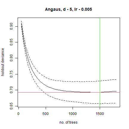
This model was built with the default 10-fold cross-validation. The solid black curve is the mean, and the dotted curves about 1 standard error, for the changes in predictive deviance (ie as measured on the excluded folds of the cross-validation). The red line shows the minimum of the mean, and the green line the number of trees at which that occurs. The final model that is returned in the model object is built on the full data set, using the number of trees identified as optimal.
The returned object is a list (see R documentation if you don’t know what that is), and the names of the components can be seen by typing:
To pull out one component of the list, use a number (angaus.tc5.lr01[[29]]) or name (angaus.tc5.lr01$cv.statistics) - but be careful, some are as big as the dataset, e.g. there will be 1000 fitted values. Find this by typing
length(angaus.tc5.lr01$fitted)
The way we organise our functions is to return exactly what Ridgeway’s function in the gbm package returned, plus extra things that are relevant to our code. You will see by looking at the final parts of the gbm.step code that we have added components 25 onwards, that is, from gbm.call on. See the gbm documentation for what his parts comprise. Ours are:
gbm.call - A list containing the details of the original call to gbm.step
fitted - The fitted values from the final tree, on the response scale
fitted.vars - The variance of the fitted values, on the response scale
residuals - The residuals for the fitted values, on the response scale
contributions - The relative importance of the variables, produced from the gbm summary function
self.statistics - The relevant set of evaluation statistics, calculated on the fitted values - i.e. this is only interesting in so far as it demonstrates “evaluation” (i.e. fit) on the training data. It should NOT be reported as the model predictive performance.
cv.statistics These are the most appropriate evaluation statistics. We calculate each statistic within each fold (at the identified optimal number of trees that is calculated on the mean change in predictive deviance over all folds), then present here the mean and standard error of those fold-based statistics.
weights - the weights used in fitting the model (by default, “1” for each observation - i.e. equal weights).
trees.fitted - A record of the number of trees fitted at each step in the stagewise fitting; only relevant for later calculations
training.loss.values - The stagewise changes in deviance on the training data
cv.values - the mean of the CV estimates of predictive deviance, calculated at each step in the stagewise process - this and the next are used in the plot shown above
cv.loss.ses - standard errors in CV estimates of predictive deviance at each step in the stagewise process
cv.loss.matrix - the matrix of values from which cv.values were calculated - as many rows as folds in the CV
cv.roc.matrix - as above, but the values in it are area under the curve estimated on the excluded data, instead of deviance in the cv.loss.matrix.
You can look at variable importance with the summary function
names(angaus.tc5.lr01)
##  [1] "initF"                "fit"                  "train.error"
##  [4] "valid.error"          "oobag.improve"        "trees"
##  [7] "c.splits"             "bag.fraction"         "distribution"
## [10] "interaction.depth"    "n.minobsinnode"       "num.classes"
## [13] "n.trees"              "nTrain"               "train.fraction"
## [16] "response.name"        "shrinkage"            "var.levels"
## [19] "var.monotone"         "var.names"            "var.type"
## [22] "verbose"              "data"                 "Terms"
## [25] "cv.folds"             "call"                 "m"
## [28] "gbm.call"             "fitted"               "fitted.vars"
## [31] "residuals"            "contributions"        "self.statistics"
## [34] "cv.statistics"        "weights"              "trees.fitted"
## [37] "training.loss.values" "cv.values"            "cv.loss.ses"
## [40] "cv.loss.matrix"       "cv.roc.matrix"
summary(angaus.tc5.lr01)
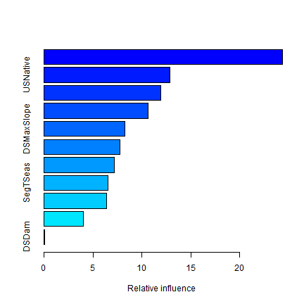
##                   var     rel.inf
## SegSumT       SegSumT 24.38814078
## USNative     USNative 12.87889951
## DSDist         DSDist 11.90091735
## Method         Method 10.61370646
## DSMaxSlope DSMaxSlope  8.23624294
## USRainDays USRainDays  7.77965715
## USSlope       USSlope  7.17173978
## SegTSeas     SegTSeas  6.51684705
## USAvgT         USAvgT  6.36887470
## SegLowFlow SegLowFlow  4.05900034
## DSDam           DSDam  0.08597395
Choosing the settings
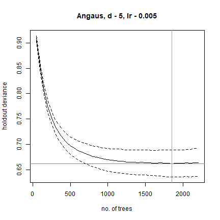
The above was a first guess at settings, using rules of thumb discussed in Elith et al. (2008). It made a model with only 650 trees, so our next step would be to reduce the lr. For example, try lr = 0.005, to aim for over 1000 trees:
angaus.tc5.lr005 <- gbm.step(data=Anguilla_train, gbm.x = 3:13, gbm.y = 2,
                      family = "bernoulli", tree.complexity = 5,
                      learning.rate = 0.005, bag.fraction = 0.5)
##
##
##  GBM STEP - version 2.9
##
## Performing cross-validation optimisation of a boosted regression tree model
## for Angaus and using a family of bernoulli
## Using 1000 observations and 11 predictors
## creating 10 initial models of 50 trees
##
##  folds are stratified by prevalence
## total mean deviance =  1.0063
## tolerance is fixed at  0.001
## ntrees resid. dev.
## 50    0.9092
## now adding trees...
## 100   0.8483
## 150   0.8069
## 200   0.7758
## 250   0.7527
## 300   0.7355
## 350   0.7224
## 400   0.7123
## 450   0.7043
## 500   0.6972
## 550   0.6929
## 600   0.6886
## 650   0.6853
## 700   0.6824
## 750   0.6796
## 800   0.6766
## 850   0.6748
## 900   0.6728
## 950   0.6713
## 1000   0.6697
## 1050   0.6688
## 1100   0.6679
## 1150   0.6675
## 1200   0.6669
## 1250   0.6654
## 1300   0.6655
## 1350   0.6648
## 1400   0.6645
## 1450   0.6648
## 1500   0.6643
## 1550   0.6642
## 1600   0.6636
## 1650   0.6633
## 1700   0.6639
## 1750   0.6632
## 1800   0.6628
## 1850   0.6624
## 1900   0.663
## 1950   0.6627
## 2000   0.6629
## 2050   0.6637
## 2100   0.6635
## 2150   0.6645
## 2200   0.6643
## fitting final gbm model with a fixed number of 1850 trees for Angaus
##
## mean total deviance = 1.006
## mean residual deviance = 0.388
##
## estimated cv deviance = 0.662 ; se = 0.026
##
## training data correlation = 0.832
## cv correlation =  0.597 ; se = 0.019
##
## training data AUC score = 0.976
## cv AUC score = 0.879 ; se = 0.014
##
## elapsed time -  0.4 minutes
To more broadly explore whether other settings perform better, and assuming that these are the only data available, you could either split the data into a training and testing set or use the cross-validation results. You could systematically alter tc, lr and the bag fraction and compare the results. See the later section on prediction to find out how to predict to independent data and calculate relevant statistics.
Alternative ways to fit models
The step function above is slower than just fitting one model and finding a minimum. If this is a problem, you could use our gbm.holdout code - this combines from the gbm package in ways we find useful. We tend to prefer gbm.step, especially when modelling many species, because it automatically finds the optimal number of trees. Alternatively, the gbm.fixed code allows you to fit a model of a set number of trees; this can be used, as in Elith et al. (2008), to predict to new data (see later section).
section{Simplifying the model
For a discussion of simplification see Appendix 2 of the online supplement to Elith et al (2008). Simplification builds many models, so it can be slow. For example, the code below took a few minutes to run on a modern laptop. In it we assess the value in simplifying the model built with a lr of 0.005, but only test dropping up to 5 variables (the “n.drop” argument; the default is an automatic rule so it continues until the average change in predictive deviance exceeds its original standard error as calculated in gbm.step).
angaus.simp <- gbm.simplify(angaus.tc5.lr005, n.drops = 5)
## gbm.simplify - version 2.9
## simplifying gbm.step model for Angaus with 11 predictors and 1000 observations
## original deviance = 0.6624(0.0263)
## a fixed number of 5 drops will be tested
## creating initial models...
## dropping predictor: 1 2 3 4 5
## processing final dropping of variables with full data
## 1-DSDam
## 2-SegLowFlow
## 3-USAvgT
## 4-SegTSeas
## 5-DSMaxSlope
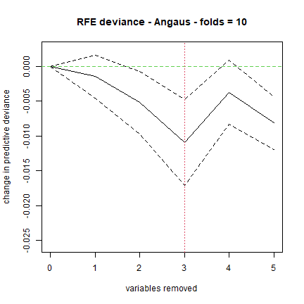
For our run, this estimated that the optimal number of variables to drop was 1; yours could be slightly different:
You can use the number indicated by the red vertical line, or look at
the results in the angaus.simp object Now make a model with 1 predictor
dropped, by indicating to the gbm.step call the relevant number of
predictor(s) from the predictor list in the angaus.simp object - see
highlights, below, in which we indicate we want to drop 1 variable by
calling the second vector of predictor columns in the pred list, using
[[1]]:
angaus.tc5.lr005.simp <- gbm.step(Anguilla_train,
                   gbm.x=angaus.simp$pred.list[[1]], gbm.y=2,
                   tree.complexity=5, learning.rate=0.005)
##
##
##  GBM STEP - version 2.9
##
## Performing cross-validation optimisation of a boosted regression tree model
## for Angaus and using a family of bernoulli
## Using 1000 observations and 10 predictors
## creating 10 initial models of 50 trees
##
##  folds are stratified by prevalence
## total mean deviance =  1.0063
## tolerance is fixed at  0.001
## ntrees resid. dev.
## 50    0.9082
## now adding trees...
## 100   0.8502
## 150   0.8115
## 200   0.7834
## 250   0.7627
## 300   0.7472
## 350   0.7355
## 400   0.7268
## 450   0.72
## 500   0.7139
## 550   0.7099
## 600   0.7065
## 650   0.7037
## 700   0.7011
## 750   0.6998
## 800   0.6986
## 850   0.6974
## 900   0.6969
## 950   0.6961
## 1000   0.695
## 1050   0.6948
## 1100   0.6947
## 1150   0.6936
## 1200   0.6934
## 1250   0.6937
## 1300   0.6936
## 1350   0.693
## 1400   0.6927
## 1450   0.693
## 1500   0.6925
## 1550   0.6935
## 1600   0.6947
## 1650   0.6947
## 1700   0.6953
## 1750   0.696
## 1800   0.6962
## fitting final gbm model with a fixed number of 1500 trees for Angaus
##
## mean total deviance = 1.006
## mean residual deviance = 0.419
##
## estimated cv deviance = 0.692 ; se = 0.035
##
## training data correlation = 0.813
## cv correlation =  0.574 ; se = 0.035
##
## training data AUC score = 0.971
## cv AUC score = 0.871 ; se = 0.012
##
## elapsed time -  0.29 minutes
This has now made a new model (angaus.tc5.lr005.simp) with the same list components as described earlier. We could continue to use it, but given that we don’t particularly want a more simple model (our view is that, in a dataset of this size, included variables that contribute little are acceptable), we won’t use it further.
Plotting the functions and fitted values from the model
The fitted functions from a BRT model created from any of our functions can be plotted using gbm.plot. If you want to plot all variables on one sheet first set up a graphics device with the right set-up - here we will make one with 3 rows and 4 columns:
gbm.plot(angaus.tc5.lr005, n.plots=11, plot.layout=c(4, 3), write.title = FALSE)
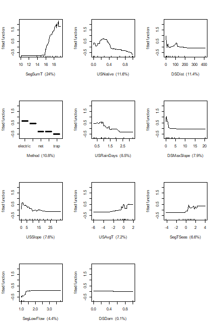
Additional arguments to this function allow for making a smoothed representation of the plot, allowing different vertical scales for each variable, omitting (and formatting) the rugs, and plotting a single variable.
Depending on the distribution of observations within the environmental space, fitted functions can give a misleading indication about the distribution of the fitted values in relation to each predictor. The function gbm.plot.fits has been provided to plot the fitted values in relation to each of the predictors used in the model.
gbm.plot.fits(angaus.tc5.lr005)
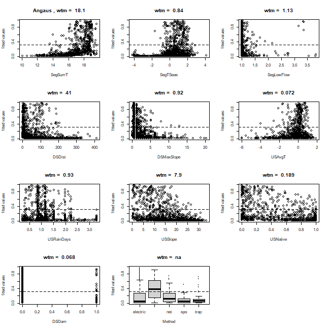
This has options that allow for the plotting of all fitted values or of fitted values only for positive observations, or the plotting of fitted values in factor type graphs that are much quicker to print. Values above each graph indicate the weighted mean of fitted values in relation to each non-factor predictor.
Interrogate and plot the interactions
This code assesses the extent to which pairwise interactions exist in the data.
find.int <- gbm.interactions(angaus.tc5.lr005).
The returned object, here named test.int, is a list. The first 2
components summarise the results, first as a ranked list of the 5 most
important pairwise interactions, and the second tabulating all pairwise
interactions. The variable index numbers in `rank.list can be
used for plotting.
find.int <- gbm.interactions(angaus.tc5.lr005)
## gbm.interactions - version 2.9
## Cross tabulating interactions for gbm model with 11 predictors
## 1 2 3 4 5 6 7 8 9 10
find.int$interactions
##            SegSumT SegTSeas SegLowFlow DSDist DSMaxSlope USAvgT USRainDays
## SegSumT          0     4.21       0.20  21.00       1.49  12.90      25.25
## SegTSeas         0     0.00       1.88   9.15       1.29   0.52       1.35
## SegLowFlow       0     0.00       0.00   0.51       0.75   1.65       0.11
## DSDist           0     0.00       0.00   0.00       0.06   0.11       4.88
## DSMaxSlope       0     0.00       0.00   0.00       0.00   1.33       0.38
## USAvgT           0     0.00       0.00   0.00       0.00   0.00       0.47
## USRainDays       0     0.00       0.00   0.00       0.00   0.00       0.00
## USSlope          0     0.00       0.00   0.00       0.00   0.00       0.00
## USNative         0     0.00       0.00   0.00       0.00   0.00       0.00
## DSDam            0     0.00       0.00   0.00       0.00   0.00       0.00
## Method           0     0.00       0.00   0.00       0.00   0.00       0.00
##            USSlope USNative DSDam Method
## SegSumT       4.03     7.39  0.04  13.87
## SegTSeas      0.24     0.67  0.00   1.46
## SegLowFlow    1.35     0.36  0.00   0.82
## DSDist        1.07     1.47  0.00   2.33
## DSMaxSlope    0.86     2.88  0.00   0.39
## USAvgT        0.19     2.31  0.00   0.82
## USRainDays    0.46     3.67  0.02   2.78
## USSlope       0.00     2.00  0.00   3.82
## USNative      0.00     0.00  0.00   2.88
## DSDam         0.00     0.00  0.00   0.00
## Method        0.00     0.00  0.00   0.00
find.int$rank.list
##   var1.index var1.names var2.index var2.names int.size
## 1          7 USRainDays          1    SegSumT    25.25
## 2          4     DSDist          1    SegSumT    21.00
## 3         11     Method          1    SegSumT    13.87
## 4          6     USAvgT          1    SegSumT    12.90
## 5          4     DSDist          2   SegTSeas     9.15
## 6          9   USNative          1    SegSumT     7.39
You can plot pairwise interactions like this:
gbm.perspec(angaus.tc5.lr005, 7, 1, y.range=c(15,20), z.range=c(0,0.6))
## maximum value = 0.62
## Warning in persp.default(x = x.var, y = y.var, z = pred.matrix, zlim =
## z.range, : surface extends beyond the box
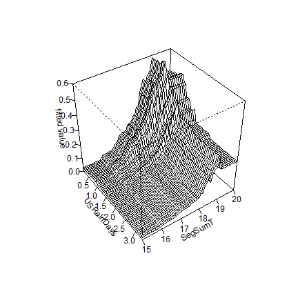
Additional options allow specifications of label names, rotations of the 3D graph and so on.
Predicting to new data
If you want to predict to a set of sites (rather than to a whole map), the general procedure is to set up a data.frame with rows for sites and columns for the variables that are in your model. R is case sensitive; the names need to exactly match those in the model. Other columns such as site IDs etc can also exist in the data.frame (and are ignored).
Our dataset for predicting to sites is in a file called Anguilla_test. The “Method” column needs to be converted to a factor, with levels matching those in the modelling data. To make predictions to sites from the BRT model use predict (or predict.gbm) from the gbm package
The predictions are in a vector called preds. These are evaluation sites, and have observations in column 1 (named Angaus_obs).
They are independent of the model building set and were used for an evaluation with independent data. Note that the calc.deviance function has different formulae for different distributions of data; the default is binomial, so we didn’t specify it in the call
data(Anguilla_test)
library(gbm)
preds <- predict.gbm(angaus.tc5.lr005, Anguilla_test,
         n.trees=angaus.tc5.lr005$gbm.call$best.trees, type="response")
calc.deviance(obs=Anguilla_test$Angaus_obs, pred=preds, calc.mean=TRUE)
## [1] 0.7420087
d <- cbind(Anguilla_test$Angaus_obs, preds)
pres <- d[d[,1]==1, 2]
abs <- d[d[,1]==0, 2]
e <- evaluate(p=pres, a=abs)
e
## class          : ModelEvaluation
## n presences    : 107
## n absences     : 393
## AUC            : 0.8610972
## cor            : 0.5263345
## max TPR+TNR at : 0.1021038
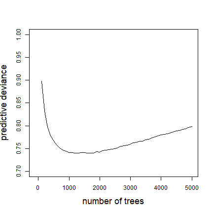
One useful feature of prediction in gbm is you can predict to a varying number of trees. See the highlighted code below to how to predict to a vector of trees. The full set of code here shows how to make one of the graphed lines from Fig. 2 in our paper, using a model of 5000 trees developed with gbm.fixed
angaus.5000 <- gbm.fixed(data=Anguilla_train, gbm.x=3:13, gbm.y=2,
               learning.rate=0.005, tree.complexity=5, n.trees=5000)
## [1] fitting gbm model with a fixed number of 5000 trees for Angaus
## [1] total deviance = 1006.33
## [1] residual deviance = 203.21
tree.list <- seq(100, 5000, by=100)
pred <- predict.gbm(angaus.5000, Anguilla_test, n.trees=tree.list, "response")
Note that the code above makes a matrix, with each column being the predictions from the model angaus.5000 to the number of trees specified by that element of tree.list - for example, the predictions in column 5 are for tree.list[5] = 500 trees. Now to calculate the deviance of all these results, and plot them:
angaus.pred.deviance <- rep(0,50)
for (i in 1:50) {
   angaus.pred.deviance[i] <- calc.deviance(Anguilla_test$Angaus_obs,
                               pred[,i], calc.mean=TRUE)
}
plot(tree.list, angaus.pred.deviance, ylim=c(0.7,1), xlim=c(-100,5000),
     type='l', xlab="number of trees", ylab="predictive deviance",
     cex.lab=1.5)
Spatial prediction
Here we show how to predict to a whole map (technically to a RasterLayer
object) using the predict version in the raster package. The
predictor variables are available as a RasterBrick (multi-layered
raster) in Anguilla_grids.
data(Anguilla_grids)
plot(Anguilla_grids)
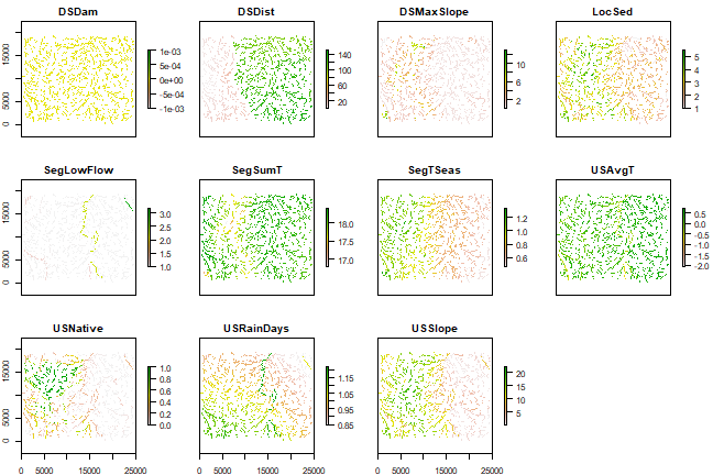
There is (obviously) no grid for fishing method. We create a data.frame with a constant value (of class ‘factor’) and pass that on to the predict function.
Method <- factor('electric', levels = levels(Anguilla_train$Method))
add <- data.frame(Method)
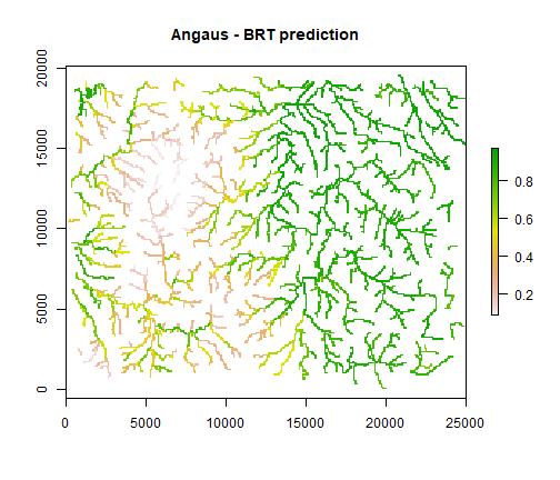
p <- predict(Anguilla_grids, angaus.tc5.lr005, const=add,
n.trees=angaus.tc5.lr005$gbm.call$best.trees, type="response")
p <- mask(p, raster(Anguilla_grids, 1))
plot(p, main='Angaus - BRT prediction')
Further reading
Elith, J., Leathwick, J.R., and Hastie, T. (2008). Boosted regression trees - a new technique for modelling ecological data. Journal of Animal Ecology