Modeling methods
Types of algorithms and data used in examples
A large number of algorithms has been used in species distribution modeling. They can be classified as ‘profile’, ‘regression’, and ‘machine learning’ methods. Profile methods only consider ‘presence’ data, not absence or background data. Regression and machine learning methods use both presence and absence or background data. The distinction between regression and machine learning methods is not sharp, but it is perhaps still useful as way to classify models. Another distinction that one can make is between presence-only and presence-absence models. Profile methods are always presence-only, other methods can be either, depending if they are used with survey-absence or with pseudo-absence/background data. An entirely different class of models consists of models that only, or primarily, use the geographic location of known occurrences, and do not rely on the values of predictor variables at these locations. We refer to these models as ‘geographic models’. Below we discuss examples of these different types of models.
First recreate the data we have used so far.
library(dismo)
library(maptools)
data(wrld_simpl)
predictors <- stack(list.files(file.path(system.file(package="dismo"), 'ex'), pattern='grd$', full.names=TRUE ))
file <- file.path(system.file(package="dismo"), "ex/bradypus.csv")
bradypus <- read.table(file,  header=TRUE,  sep=',')
bradypus <- bradypus[,-1]
presvals <- extract(predictors, bradypus)
set.seed(0)
backgr <- randomPoints(predictors, 500)
absvals <- extract(predictors, backgr)
pb <- c(rep(1, nrow(presvals)), rep(0, nrow(absvals)))
sdmdata <- data.frame(cbind(pb, rbind(presvals, absvals)))
sdmdata[,'biome'] <- as.factor(sdmdata[,'biome'])
We will use the same data to illustrate all models, except that some models cannot use categorical variables. So for those models we drop the categorical variables from the predictors stack.
pred_nf <- dropLayer(predictors, 'biome')
We use the Bradypus data for presence of a species. First we make a
training and a testing set.
set.seed(0)
group <- kfold(bradypus, 5)
pres_train <- bradypus[group != 1, ]
pres_test <- bradypus[group == 1, ]
To speed up processing, let’s restrict the predictions to a more restricted area (defined by a rectangular extent):
ext <- extent(-90, -32, -33, 23)
Background data for training and a testing set. The first layer in the
RasterStack is used as a ‘mask’. That ensures that random points only
occur within the spatial extent of the rasters, and within cells that
are not NA, and that there is only a single absence point per cell.
Here we further restrict the background points to be within 12.5% of our
specified extent ‘ext’.
set.seed(10)
backg <- randomPoints(pred_nf, n=1000, ext=ext, extf = 1.25)
colnames(backg) = c('lon', 'lat')
group <- kfold(backg, 5)
backg_train <- backg[group != 1, ]
backg_test <- backg[group == 1, ]
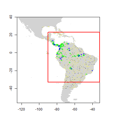
r <- raster(pred_nf, 1)
plot(!is.na(r), col=c('white', 'light grey'), legend=FALSE)
plot(ext, add=TRUE, col='red', lwd=2)
points(backg_train, pch='-', cex=0.5, col='yellow')
points(backg_test, pch='-',  cex=0.5, col='black')
points(pres_train, pch= '+', col='green')
points(pres_test, pch='+', col='blue')
Profile methods
The three methods described here, Bioclim, Domain, and Mahal. These methods are implemented in the dismo package, and the procedures to use these models are the same for all three.
Bioclim
The BIOCLIM algorithm has been extensively used for species distribution modeling. BIOCLIM is a classic ‘climate-envelope-model’ (Booth et al., 2014). Although it generally does not perform as good as some other modeling methods (Elith et al. 2006), particularly in the context of climate change (Hijmans and Graham, 2006), it is still used, among other reasons because the algorithm is easy to understand and thus useful in teaching species distribution modeling. The BIOCLIM algorithm computes the similarity of a location by comparing the values of environmental variables at any location to a percentile distribution of the values at known locations of occurrence (‘training sites’). The closer to the 50th percentile (the median), the more suitable the location is. The tails of the distribution are not distinguished, that is, 10 percentile is treated as equivalent to 90 percentile. In the ‘dismo’ implementation, the values of the upper tail values are transformed to the lower tail, and the minimum percentile score across all the environmental variables is used (i.e., BIOCLIM uses an approach like Liebig’s law of the minimum). This value is subtracted from 1 and then multiplied with two so that the results are between 0 and 1. The reason for scaling this way is that the results become more like that of other distribution modeling methods and are thus easier to interpret. The value 1 will rarely be observed as it would require a location that has the median value of the training data for all the variables considered. The value 0 is very common as it is assigned to all cells with a value of an environmental variable that is outside the percentile distribution (the range of the training data) for at least one of the variables.
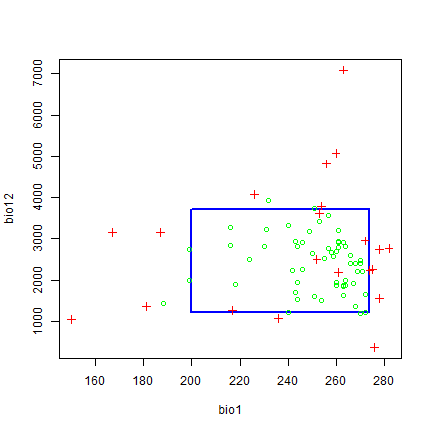
Earlier on, we fitted a Bioclim model using data.frame with each row representing the environmental data at known sites of presence of a species. Here we fit a bioclim model simply using the predictors and the occurrence points (the function will do the extracting for us).
bc <- bioclim(pred_nf, pres_train)
plot(bc, a=1, b=2, p=0.85)
We evaluate the model in a similar way, by providing presence and background (absence) points, the model, and a RasterStack:
e <- evaluate(pres_test, backg_test, bc, pred_nf)
e
## class          : ModelEvaluation
## n presences    : 23
## n absences     : 200
## AUC            : 0.6890217
## cor            : 0.1765706
## max TPR+TNR at : 0.08592151
Find a threshold
tr <- threshold(e, 'spec_sens')
tr
## [1] 0.08592151
And we use the RasterStack with predictor variables to make a prediction to a RasterLayer:
pb <- predict(pred_nf, bc, ext=ext, progress='')
pb
## class : RasterLayer
## dimensions : 112, 116, 12992 (nrow, ncol, ncell)
## resolution : 0.5, 0.5 (x, y)
## extent : -90, -32, -33, 23 (xmin, xmax, ymin, ymax)
## crs : +proj=longlat +datum=WGS84 +no_defs
## source : memory
## names : layer
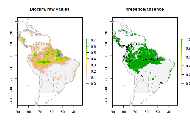
## values : 0, 0.7096774 (min, max)
par(mfrow=c(1,2))
plot(pb, main='Bioclim, raw values')
plot(wrld_simpl, add=TRUE, border='dark grey')
plot(pb > tr, main='presence/absence')
plot(wrld_simpl, add=TRUE, border='dark grey')
points(pres_train, pch='+')
Please note the order of the arguments in the predict function. In the
example above, we used predict(pred\_nf, bc) (first the RasterStack,
then the model object), which is little bit less efficient than
predict(bc, pred_nf) (first the model, than the RasterStack). The reason
for using the order we have used, is that this will work for all models,
whereas the other option only works for the models defined in the dismo
package, such as Bioclim, Domain, and Maxent, but not for models defined
in other packages (random forest, boosted regression trees, glm, etc.).
Domain
The Domain algorithm (Carpenter et al. 1993) has been extensively used for species distribution modeling. It did not perform very well in a model comparison (Elith et al. 2006) and very poorly when assessing climate change effects (Hijmans and Graham, 2006). The Domain algorithm computes the Gower distance between environmental variables at any location and those at any of the known locations of occurrence (‘training sites’).
The distance between the environment at point A and those of the known occurrences for a single climate variable is calculated as the absolute difference in the values of that variable divided by the range of the variable across all known occurrence points (i.e., the distance is scaled by the range of observations). For each variable the minimum distance between a site and any of the training points is taken. The Gower distance is then the mean of these distances over all environmental variables. The algorithm assigns to a place the distance to the closest known occurrence (in environmental space).
To integrate over environmental variables, the distance to any of the variables is used. This distance is subtracted from one, and (in this R implementation) values below zero are truncated so that the scores are between 0 (low) and 1 (high).
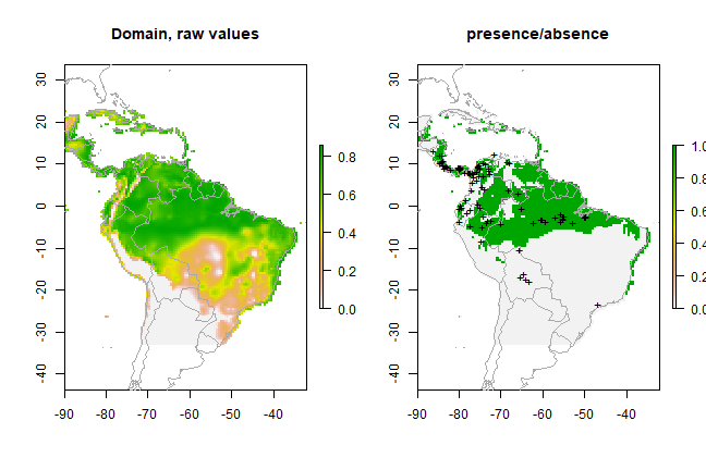
Below we fit a domain model, evaluate it, and make a prediction. We map the prediction, as well as a map subjectively classified into presence / absence.
dm <- domain(pred_nf, pres_train)
e <- evaluate(pres_test, backg_test, dm, pred_nf)
e
## class          : ModelEvaluation
## n presences    : 23
## n absences     : 200
## AUC            : 0.7097826
## cor            : 0.2138087
## max TPR+TNR at : 0.7107224
pd = predict(pred_nf, dm, ext=ext, progress='')
par(mfrow=c(1,2))
plot(pd, main='Domain, raw values')
plot(wrld_simpl, add=TRUE, border='dark grey')
tr <- threshold(e, 'spec_sens')
plot(pd > tr, main='presence/absence')
plot(wrld_simpl, add=TRUE, border='dark grey')
points(pres_train, pch='+')
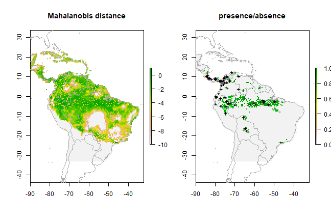
Mahalanobis distance
The mahal function implements a species distribution model based on
the Mahalanobis distance (Mahalanobis, 1936). Mahalanobis distance takes
into account the correlations of the variables in the data set, and it
is not dependent on the scale of measurements.
mm <- mahal(pred_nf, pres_train)
e <- evaluate(pres_test, backg_test, mm, pred_nf)
e
## class          : ModelEvaluation
## n presences    : 23
## n absences     : 200
## AUC            : 0.7686957
## cor            : 0.1506777
## max TPR+TNR at : 0.1116504
pm = predict(pred_nf, mm, ext=ext, progress='')
par(mfrow=c(1,2))
pm[pm < -10] <- -10
plot(pm, main='Mahalanobis distance')
plot(wrld_simpl, add=TRUE, border='dark grey')
tr <- threshold(e, 'spec_sens')
plot(pm > tr, main='presence/absence')
plot(wrld_simpl, add=TRUE, border='dark grey')
points(pres_train, pch='+')
Classical regression models
The remaining models need to be fit with presence and absence
(background) data. With the exception of ‘maxent’, we cannot fit the
model with a RasterStack and points. Instead, we need to extract the
environmental data values ourselves, and fit the models with these
values.
train <- rbind(pres_train, backg_train)
pb_train <- c(rep(1, nrow(pres_train)), rep(0, nrow(backg_train)))
envtrain <- extract(predictors, train)
envtrain <- data.frame( cbind(pa=pb_train, envtrain) )
envtrain[,'biome'] = factor(envtrain[,'biome'], levels=1:14)
head(envtrain)
##   pa bio1 bio12 bio16 bio17 bio5 bio6 bio7 bio8 biome
## 1  1  263  1639   724    62  338  191  147  261     1
## 2  1  263  1639   724    62  338  191  147  261     1
## 3  1  253  3624  1547   373  329  150  179  271     1
## 4  1  243  1693   775   186  318  150  168  264     1
## 5  1  252  2501  1081   280  326  154  172  270     1
## 6  1  240  1214   516   146  317  150  168  261     2
testpres <- data.frame( extract(predictors, pres_test) )
testbackg <- data.frame( extract(predictors, backg_test) )
testpres[ ,'biome'] = factor(testpres[ ,'biome'], levels=1:14)
testbackg[ ,'biome'] = factor(testbackg[ ,'biome'], levels=1:14)
Generalized Linear Models
A generalized linear model (GLM) is a generalization of ordinary least
squares regression. Models are fit using maximum likelihood and by
allowing the linear model to be related to the response variable via a
link function and by allowing the magnitude of the variance of each
measurement to be a function of its predicted value. Depending on how a
GLM is specified it can be equivalent to (multiple) linear regression,
logistic regression or Poisson regression. See Guisan et al (2002)
for an overview of the use of GLM in species distribution modeling.
In R, GLM is implemented in the ‘glm’ function, and the link function and error distribution are specified with the ‘family’ argument. Examples are:
family = binomial(link = "logit")
family = gaussian(link = "identity")
family = poisson(link = "log")
Here we fit two basic glm models. All variables are used, but without interaction terms.
# logistic regression:
gm1 <- glm(pa ~ bio1 + bio5 + bio6 + bio7 + bio8 + bio12 + bio16 + bio17,
            family = binomial(link = "logit"), data=envtrain)
summary(gm1)
##
## Call:
## glm(formula = pa ~ bio1 + bio5 + bio6 + bio7 + bio8 + bio12 +
##     bio16 + bio17, family = binomial(link = "logit"), data = envtrain)
##
## Deviance Residuals:
##      Min        1Q    Median        3Q       Max
## -1.73818  -0.49933  -0.23999  -0.06579   2.91501
##
## Coefficients:
##               Estimate Std. Error z value Pr(>|z|)
## (Intercept)  3.0540581  1.5774812   1.936  0.05286 .
## bio1         0.0906378  0.0577068   1.571  0.11626
## bio5         0.2403921  0.2520843   0.954  0.34028
## bio6        -0.3227360  0.2541727  -1.270  0.20417
## bio7        -0.3212603  0.2528026  -1.271  0.20380
## bio8        -0.0133843  0.0255062  -0.525  0.59976
## bio12        0.0020951  0.0006931   3.023  0.00250 **
## bio16       -0.0023747  0.0014546  -1.633  0.10256
## bio17       -0.0047152  0.0015473  -3.047  0.00231 **
## ---
## Signif. codes:  0 '***' 0.001 '**' 0.01 '*' 0.05 '.' 0.1 ' ' 1
##
## (Dispersion parameter for binomial family taken to be 1)
##
##     Null deviance: 596.69  on 892  degrees of freedom
## Residual deviance: 449.77  on 884  degrees of freedom
## AIC: 467.77
##
## Number of Fisher Scoring iterations: 8
coef(gm1)
##  (Intercept)         bio1         bio5         bio6         bio7         bio8
##  3.054058115  0.090637822  0.240392091 -0.322736029 -0.321260278 -0.013384258
##        bio12        bio16        bio17
##  0.002095136 -0.002374688 -0.004715157
gm2 <- glm(pa ~ bio1+bio5 + bio6 + bio7 + bio8 + bio12 + bio16 + bio17,
            family = gaussian(link = "identity"), data=envtrain)
evaluate(testpres, testbackg, gm1)
## class          : ModelEvaluation
## n presences    : 23
## n absences     : 200
## AUC            : 0.8156522
## cor            : 0.308183
## max TPR+TNR at : -2.565312
ge2 <- evaluate(testpres, testbackg, gm2)
ge2
## class          : ModelEvaluation
## n presences    : 23
## n absences     : 200
## AUC            : 0.7886957
## cor            : 0.3629842
## max TPR+TNR at : 0.08711959
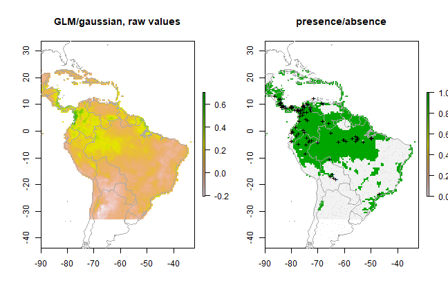
pg <- predict(predictors, gm2, ext=ext)
par(mfrow=c(1,2))
plot(pg, main='GLM/gaussian, raw values')
plot(wrld_simpl, add=TRUE, border='dark grey')
tr <- threshold(ge2, 'spec_sens')
plot(pg > tr, main='presence/absence')
plot(wrld_simpl, add=TRUE, border='dark grey')
points(pres_train, pch='+')
points(backg_train, pch='-', cex=0.25)
Generalized Additive Models
Generalized additive models (GAMs; Hastie and Tibshirani, 1990; Wood, 2006) are an extension to GLMs. In GAMs, the linear predictor is the sum of smoothing functions. This makes GAMs very flexible, and they can fit very complex functions. It also makes them very similar to machine learning methods. In R, GAMs are implemented in the ‘mgcv’ package.
Machine learning methods
Machine learning models, are non-parametric flexible regression models. Methods include Artifical Neural Networks (ANN), Random Forests, Boosted Regression Trees, and Support Vector Machines. Through the dismo package you can also use the Maxent program, that implements the most widely used method (maxent) in species distribution modeling. Breiman (2001a) provides a accessible introduction to machine learning, and how it contrasts with ‘classical statistics’ (model based probabilistic inference). Hastie et al., 2009 provide what is probably the most extensive overview of these methods.
All the model fitting methods discussed here can be tuned in several ways. We do not explore that here, and only show the general approach. If you want to use one of the methods, then you should consult the R help pages (and other sources) to find out how to best implement the model fitting procedure.
Maxent
MaxEnt (short for “Maximum Entropy”; Phillips et al., 2006) is the most widely used SDM algorithm. Elith et al. (2010) provide an explanation of the algorithm (and software) geared towards ecologists. MaxEnt is available as a stand-alone Java program. Dismo has a function ‘maxent’ that communicates with this program.
Because MaxEnt is implemented in dismo you can fit it like the profile methods (e.g. Bioclim). That is, you can provide presence points and a RasterStack. However, you can also first fit a model, like with the other methods such as glm. But in the case of MaxEnt you cannot use the formula notation.
maxent()
## Loading required namespace: rJava
## This is MaxEnt version 3.4.3
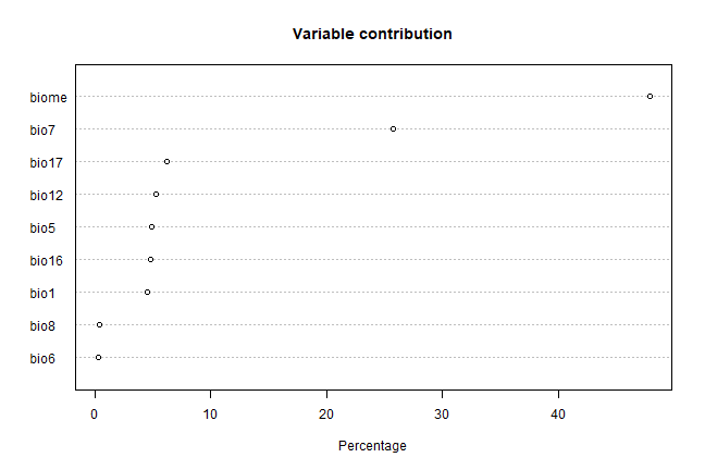
xm <- maxent(predictors, pres_train, factors='biome')
## This is MaxEnt version 3.4.3
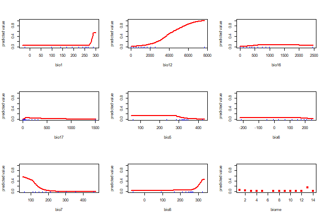
plot(xm)
A response plot:
response(xm)
e <- evaluate(pres_test, backg_test, xm, predictors)
e
## class : ModelEvaluation
## n presences : 23
## n absences : 200
## AUC : 0.8336957
## cor : 0.3789954
## max TPR+TNR at : 0.1772358
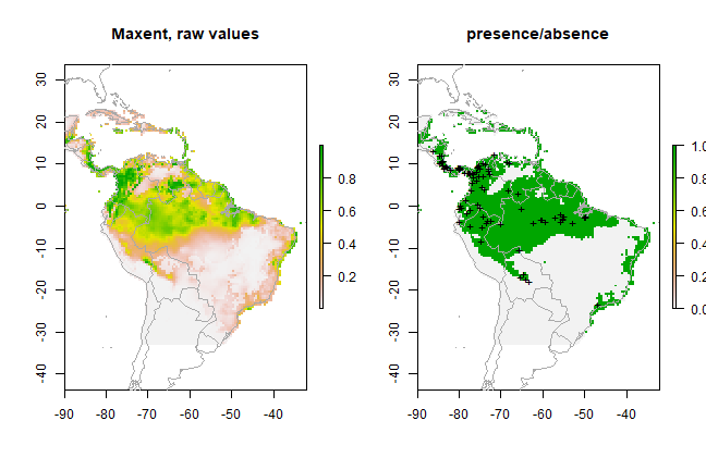
px <- predict(predictors, xm, ext=ext, progress='')
par(mfrow=c(1,2))
plot(px, main='Maxent, raw values')
plot(wrld_simpl, add=TRUE, border='dark grey')
tr <- threshold(e, 'spec_sens')
plot(px > tr, main='presence/absence')
plot(wrld_simpl, add=TRUE, border='dark grey')
points(pres_train, pch='+')
Boosted Regression Trees
Boosted Regression Trees (BRT) is, unfortunately, known by a large
number of different names. It was developed by Friedman (2001), who
referred to it as a “Gradient Boosting Machine” (GBM). It is also known
as “Gradient Boost”, “Stochastic Gradient Boosting”, “Gradient Tree
Boosting”. The method is implemented in the gbm package in R.
The article by Elith, Leathwick and Hastie (2009) describes the use of
BRT in the context of species distribution modeling. Their article is
accompanied by a number of R functions and a tutorial that have been
slightly adjusted and incorporated into the ‘dismo’ package. These
functions extend the functions in the gbm package, with the goal to
make these easier to apply to ecological data, and to enhance
interpretation. The adapted tutorial is available as an
appendix.
Random Forest
The Random Forest (Breiman, 2001b) method is an extension of Classification and regression trees (CART; Breiman et al., 1984). In R it is implemented in the function ‘randomForest’ in a package with the same name. The function randomForest can take a formula or, in two separate arguments, a data.frame with the predictor variables, and a vector with the response. If the response variable is a factor (categorical), randomForest will do classification, otherwise it will do regression. Whereas with species distribution modeling we are often interested in classification (species is present or not), it is my experience that using regression provides better results. rf1 does regression, rf2 and rf3 do classification (they are exactly the same models). See the function tuneRF for optimizing the model fitting procedure.
library(randomForest)
## randomForest 4.6-14
## Type rfNews() to see new features/changes/bug fixes.
model <- pa ~ bio1 + bio5 + bio6 + bio7 + bio8 + bio12 + bio16 + bio17
rf1 <- randomForest(model, data=envtrain)
## Warning in randomForest.default(m, y, ...): The response has five or fewer
## unique values. Are you sure you want to do regression?
model <- factor(pa) ~ bio1 + bio5 + bio6 + bio7 + bio8 + bio12 + bio16 + bio17
rf2 <- randomForest(model, data=envtrain)
rf3 <- randomForest(envtrain[,1:8], factor(pb_train))
erf <- evaluate(testpres, testbackg, rf1)
erf
## class : ModelEvaluation
## n presences : 23
## n absences : 200
## AUC : 0.8580435
## cor : 0.5010053
## max TPR+TNR at : 0.1060667
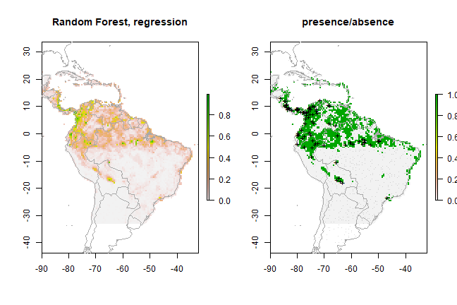
pr <- predict(predictors, rf1, ext=ext)
par(mfrow=c(1,2))
plot(pr, main='Random Forest, regression')
plot(wrld_simpl, add=TRUE, border='dark grey')
tr <- threshold(erf, 'spec_sens')
plot(pr > tr, main='presence/absence')
plot(wrld_simpl, add=TRUE, border='dark grey')
points(pres_train, pch='+')
points(backg_train, pch='-', cex=0.25)
Support Vector Machines
Support Vector Machines (SVMs; Vapnik, 1998) apply a simple linear method to the data but in a high-dimensional feature space non-linearly related to the input space, but in practice, it does not involve any computations in that high-dimensional space. This simplicity combined with state of the art performance on many learning problems (classification, regression, and novelty detection) has contributed to the popularity of the SVM (Karatzoglou et al., 2006). They were first used in species distribution modeling by Guo et al. (2005).
There are a number of implementations of svm in R. The most useful implementations in our context are probably function ‘ksvm’ in package ‘kernlab’ and the ‘svm’ function in package ‘e1071’. ‘ksvm’ includes many different SVM formulations and kernels and provides useful options and features like a method for plotting, but it lacks a proper model selection tool. The ‘svm’ function in package ‘e1071’ includes a model selection tool: the ‘tune’ function (Karatzoglou et al., 2006)
library(kernlab)
##
## Attaching package: 'kernlab'
## The following objects are masked from 'package:raster':
##
## buffer, rotated
svm <- ksvm(pa ~ bio1+bio5+bio6+bio7+bio8+bio12+bio16+bio17, data=envtrain)
esv <- evaluate(testpres, testbackg, svm)
esv
## class : ModelEvaluation
## n presences : 23
## n absences : 200
## AUC : 0.7576087
## cor : 0.3738667
## max TPR+TNR at : 0.02857293
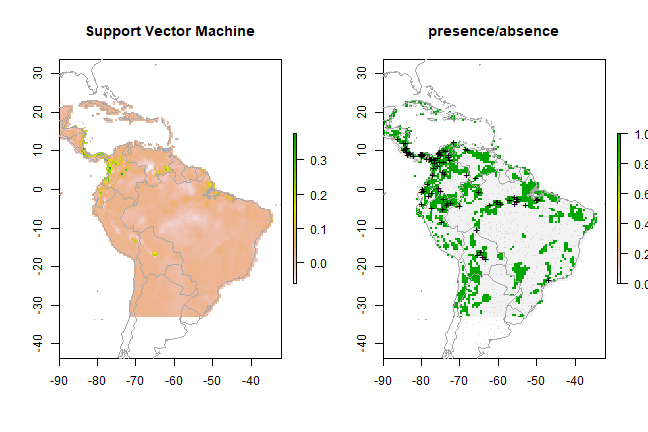
ps <- predict(predictors, svm, ext=ext)
par(mfrow=c(1,2))
plot(ps, main='Support Vector Machine')
plot(wrld_simpl, add=TRUE, border='dark grey')
tr <- threshold(esv, 'spec_sens')
plot(ps > tr, main='presence/absence')
plot(wrld_simpl, add=TRUE, border='dark grey')
points(pres_train, pch='+')
points(backg_train, pch='-', cex=0.25)
Combining model predictions
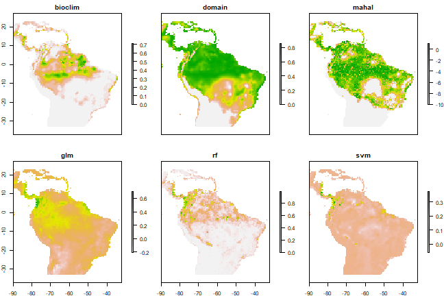
Rather than relying on a single “best” model, some auhtors (e.g. Thuillier, 2003) have argued for using many models and applying some sort of model averaging. See the biomod2 package for an implementation. You can of course implement these approaches yourself. Below is a very brief example. We first make a RasterStack of our individual model predictions:
models <- stack(pb, pd, pm, pg, pr, ps)
names(models) <- c("bioclim", "domain", "mahal", "glm", "rf", "svm")
plot(models)
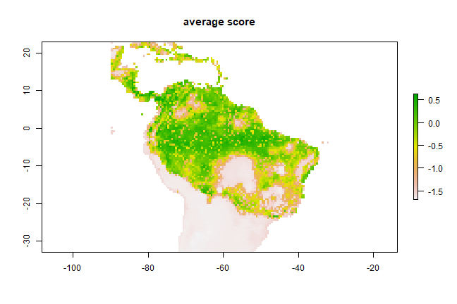
Now we can compute the simple average:
m <- mean(models)
plot(m, main='average score')
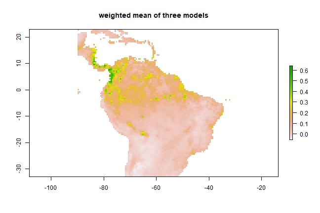
However, this is a problematic approach as the values predicted by the models are not all on the same (between 0 and 1) scale; so you may want to fix that first. Another concern could be weighting. Let’s combine three models weighted by their AUC scores. Here, to create the weights, we substract 0.5 (the random expectation) and square the result to give further weight to higher AUC values.
auc <- sapply(list(ge2, erf, esv), function(x) x@auc)
w <- (auc-0.5)^2
m2 <- weighted.mean( models[[c("glm", "rf", "svm")]], w)
plot(m2, main='weighted mean of three models')