Raster data manipulation
Introduction
In this chapter general aspects of the design of the terra package
are discussed, notably the structure of the main classes, and what they
represent. The use of the package is illustrated in subsequent sections.
terra has a large number of functions, not all of them are discussed
here, and those that are discussed are mentioned only briefly. See the
help files of the package for more information on individual functions
and help("terra-package") for an index of functions by topic.
Creating SpatRaster objects
A SpatRaster can easily be created from scratch using the function
rast. The default settings will create a global raster data
structure with a longitude/latitude coordinate reference system and 1 by
1 degree cells. You can change these settings by providing additional
arguments such as xmin, nrow, ncol, and/or crs, to the
function. You can also change these parameters after creating the
object. If you set the projection, this is only to properly define it,
not to change it. To transform a SpatRaster to another coordinate
reference system (projection) you can use the project function.
Here is an example of creating and changing a SpatRaster object ‘r’
from scratch.
library(terra)
## terra 1.9.22
# SpatRaster with the default parameters
x <- rast()
x
## class       : SpatRaster
## size        : 180, 360, 1  (nrow, ncol, nlyr)
## resolution  : 1, 1  (x, y)
## extent      : -180, 180, -90, 90  (xmin, xmax, ymin, ymax)
## coord. ref. : lon/lat WGS 84 (CRS84) (OGC:CRS84)
With some other parameters
x <- rast(ncol=36, nrow=18, xmin=-1000, xmax=1000, ymin=-100, ymax=900)
These parameters can be changed. Resolution:
res(x)
## [1] 55.55556 55.55556
res(x) <- 100
res(x)
## [1] 100 100
Change the number of columns (this affects the resolution).
ncol(x)
## [1] 20
ncol(x) <- 18
ncol(x)
## [1] 18
res(x)
## [1] 111.1111 100.0000
Set the coordinate reference system (CRS) (i.e., define the projection).
crs(x) <- "+proj=utm +zone=48 +datum=WGS84"
x
## class       : SpatRaster
## size        : 10, 18, 1  (nrow, ncol, nlyr)
## resolution  : 111.1111, 100  (x, y)
## extent      : -1000, 1000, -100, 900  (xmin, xmax, ymin, ymax)
## coord. ref. : +proj=utm +zone=48 +datum=WGS84 +units=m +no_defs
The object x created in the examples above only consists of the
raster geometry, that is, we have defined the number of rows and
columns, and where the raster is located in geographic space, but there
are no cell-values associated with it. Setting and accessing values is
illustrated below.
First another example empty raster geometry.
r <- rast(ncol=10, nrow=10)
ncell(r)
## [1] 100
hasValues(r)
## [1] FALSE
Use the ‘values’ function.
values(r) <- 1:ncell(r)
Another example.
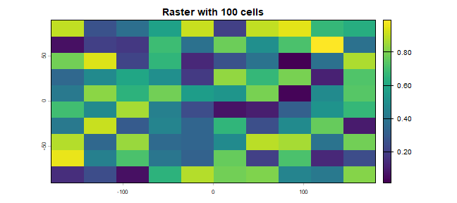
set.seed(0)
values(r) <- runif(ncell(r))

hasValues(r)
## [1] TRUE
sources(r)
## [1] ""
values(r)[1:10]
##  [1] 0.8966972 0.2655087 0.3721239 0.5728534 0.9082078 0.2016819 0.8983897
##  [8] 0.9446753 0.6607978 0.6291140
plot(r, main='Raster with 100 cells')
In some cases, for example when you change the number of columns or
rows, you will lose the values associated with the SpatRaster if
there were any (or the link to a file if there was one). The same
applies, in most cases, if you change the resolution directly (as this
can affect the number of rows or columns). Values are not lost when
changing the extent as this change adjusts the resolution, but does not
change the number of rows or columns.
hasValues(r)
## [1] TRUE
res(r)
## [1] 36 18
dim(r)
## [1] 10 10  1
# extent
ext(r)
## SpatExtent : -180, 180, -90, 90 (xmin, xmax, ymin, ymax)
Now change the maximum x coordinate of the extent (bounding box) of the
SpatRaster.
xmax(r) <- 0
hasValues(r)
## [1] TRUE
res(r)
## [1] 18 18
dim(r)
## [1] 10 10  1
And the number of columns (the values disappear)
ncol(r) <- 6
hasValues(r)
## [1] FALSE
res(r)
## [1] 30 18
dim(r)
## [1] 10  6  1
xmax(r)
## [1] 0
While we can create a SpatRaster from scratch, it is more common to
do so from a file. The terra package can use raster files in several
formats, including GeoTiff, ESRI, ENVI, and ERDAS.
A notable feature of the terra package is that it can work with
raster datasets that are stored on disk and are too large to be loaded
into memory (RAM). The package can work with large files because the
objects it creates from these files only contain information about the
structure of the data, such as the number of rows and columns, the
spatial extent, and the filename, but it does not attempt to read all
the cell values in memory. In computations with these objects, data is
processed in chunks. If no output filename is specified to a function,
and the output raster is too large to keep in memory, the results are
written to a temporary file.
Below we first we get the name of an example raster file that is
installed with the “terra” package. Do not use this system.file
construction for your own files. Just type the file name as you would do
for any other file, but don’t forget to use forward slashes as path
separators.
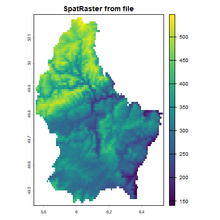
filename <- system.file("ex/elev.tif", package="terra")
basename(filename)
## [1] "elev.tif"
r <- rast(filename)
sources(r)
## [1] "C:/soft/R/R-4.5.3/library/terra/ex/elev.tif"
hasValues(r)
## [1] TRUE
plot(r, main="SpatRaster from file")
Multi-layer objects can be created in memory or from files.
Create three identical SpatRaster objects
r1 <- r2 <- r3 <- rast(nrow=10, ncol=10)
# Assign random cell values
values(r1) <- runif(ncell(r1))
values(r2) <- runif(ncell(r2))
values(r3) <- runif(ncell(r3))
Combine three SpatRasters:
s <- c(r1, r2, r3)
s
## class       : SpatRaster
## size        : 10, 10, 3  (nrow, ncol, nlyr)
## resolution  : 36, 18  (x, y)
## extent      : -180, 180, -90, 90  (xmin, xmax, ymin, ymax)
## coord. ref. : lon/lat WGS 84 (CRS84) (OGC:CRS84)
## source(s)   : memory
## names       :    lyr.1,    lyr.1,    lyr.1
## min values  : 0.013078, 0.027787, 0.063802
## max values  : 0.992684, 0.981563, 0.996077
nlyr(s)
## [1] 3
You can also create a multilayer object from a file.
filename <- system.file("ex/logo.tif", package="terra")
basename(filename)
## [1] "logo.tif"
b <- rast(filename)
b
## class       : SpatRaster
## size        : 77, 101, 3  (nrow, ncol, nlyr)
## resolution  : 1, 1  (x, y)
## extent      : 0, 101, 0, 77  (xmin, xmax, ymin, ymax)
## coord. ref. : Cartesian (Meter)
## source      : logo.tif
## colors rgb  : 1, 2, 3
## names       : red, green, blue
## min values  :   0,     0,    0
## max values  : 255,   255,  255
nlyr(b)
## [1] 3
Extract a single layer (the second one on this case)
r <- b[[2]]
Raster algebra
Many generic functions that allow for simple and elegant raster algebra
have been implemented for Raster objects, including the normal
algebraic operators such as +, -, *, /, logical
operators such as >, >=, <, ==, ! and functions like
abs, round, ceiling, floor, trunc, sqrt,
log, log10, exp, cos, sin, atan, tan,
max, min, range, prod, sum, any, all. In
these functions you can mix raster objects with numbers, as long as
the first argument is a raster object.
Create an empty SpatRaster and assign values to cells.
r <- rast(ncol=10, nrow=10)
values(r) <- 1:ncell(r)
Now some raster algebra.
s <- r + 10
s <- sqrt(s)
s <- s * r + 5
values(r) <- runif(ncell(r))
r <- round(r)
r <- r == 1
You can also use replacement functions.
#Not yet implemented
s[r] <- -0.5
s[!r] <- 5
s[s == 5] <- 15
If you use multiple SpatRaster objects (in functions where this is
relevant, such as range), these must have the same resolution and
origin. The origin of a Raster object is the point closest to (0, 0)
that you could get if you moved from a corner of a SpatRaster toward
that point in steps of the x and y resolution. Normally these
objects would also have the same extent, but if they do not, the
returned object covers the spatial intersection of the objects used.
When you use multiple multi-layer objects with different numbers or
layers, the ‘shorter’ objects are ‘recycled’. For example, if you
multiply a 4-layer object (a1, a2, a3, a4) with a
2-layer object (b1, b2), the result is a four-layer object
(a1*b1, a2*b2, a3*b1, a3*b2).
r <- rast(ncol=5, nrow=5)
values(r) <- 1
s <- c(r, r+1)
q <- c(r, r+2, r+4, r+6)
x <- r + s + q
x
## class       : SpatRaster
## size        : 5, 5, 4  (nrow, ncol, nlyr)
## resolution  : 72, 36  (x, y)
## extent      : -180, 180, -90, 90  (xmin, xmax, ymin, ymax)
## coord. ref. : lon/lat WGS 84 (CRS84) (OGC:CRS84)
## source(s)   : memory
## names       : lyr1, lyr2, lyr3, lyr4
## min values  :    3,    6,    7,   10
## max values  :    3,    6,    7,   10
Summary functions (min, max, mean, prod, sum,
median, cv, range, any, all) always return a
SpatRaster object. Perhaps this is not obvious when using functions
like min, sum or mean.
a <- mean(r,s,10)
b <- sum(r,s)
st <- c(r, s, a, b)
sst <- sum(st)
sst
## class       : SpatRaster
## size        : 5, 5, 1  (nrow, ncol, nlyr)
## resolution  : 72, 36  (x, y)
## extent      : -180, 180, -90, 90  (xmin, xmax, ymin, ymax)
## coord. ref. : lon/lat WGS 84 (CRS84) (OGC:CRS84)
## source(s)   : memory
## name        :       sum
## min value   : 17.333333
## max value   : 17.333333
Use global if you want a single number summarizing the cell values
of each layer.
global(st, 'sum')
##              sum
## lyr.1    25.0000
## lyr.1.1  25.0000
## lyr.1.2  50.0000
## lyr1    100.0000
## lyr2    108.3333
## lyr1.1   50.0000
## lyr2.1   75.0000
global(sst, 'sum')
##          sum
## sum 433.3333
‘High-level’ functions
Several ‘high level’ functions have been implemented for SpatRaster
objects. ‘High level’ functions refer to functions that you would
normally find in a computer program that supports the analysis of raster
data. Here we briefly discuss some of these functions. All these
functions work for raster datasets that cannot be loaded into memory.
See the help files for more detailed descriptions of each function.
The high-level functions have some arguments in common. The first
argument is typically a SpatRaster ‘x’ or ‘object’. It is followed
by one or more arguments specific to the function (either additional
SpatRaster objects or other arguments), followed by filename and
... arguments.
The default filename is an empty character "". If you do not specify
a filename, the default action for the function is to return a
raster object that only exists in memory. However, if the function
deems that the raster object to be created would be too large to
hold in memory, it is written to a temporary file instead.
The ... argument allows for setting additional arguments that are
relevant when writing values to a file: the file format, datatype
(e.g. integer or real values), and a to indicate whether existing files
should be overwritten.
Modifying a SpatRaster object
There are several functions that deal with modifying the spatial extent
of SpatRaster objects. The crop function lets you take a
geographic subset of a larger raster object. You can crop a
SpatRaster by providing an extent object or another spatial object
from which an extent can be extracted (objects from classes deriving
from Raster and from Spatial in the sp package). An easy way
to get an extent object is to plot a SpatRaster and then use
drawExtent to visually determine the new extent (bounding box) to
provide to the crop function.
trim crops a SpatRaster by removing the outer rows and columns
that only contain NA values. In contrast, extend adds new rows
and/or columns with NA values. The purpose of this could be to
create a new SpatRaster with the same Extent of another, larger,
SpatRaster such that they can be used together in other functions.
The merge function lets you merge 2 or more SpatRaster objects into
a single new object. The input objects must have the same resolution and
origin (such that their cells neatly fit into a single larger raster).
If this is not the case you can first adjust one of the SpatRaster
objects with aggregate/disagg or resample.
aggregate and disagg allow for changing the resolution (cell
size) of a SpatRaster object. In the case of aggregate, you need
to specify a function determining what to do with the grouped cell
values mean. It is possible to specify different (dis)aggregation
factors in the x and y direction. aggregate and disagg are the
best functions when adjusting cells size only, with an integer step
(e.g. each side 2 times smaller or larger), but in some cases that is
not possible.
For example, you may need nearly the same cell size, while shifting the
cell centers. In those cases, the resample function can be used. It
can do either nearest neighbor assignments (for categorical data) or
bilinear interpolation (for numerical data). Simple linear shifts of a
Raster object can be accomplished with the shift function or with
the extent function.
With the warp function you can transform values of SpatRaster
object to a new object with a different coordinate reference system.
Here are some simple examples.
Aggregate and disaggregate.
r <- rast()
values(r) <- 1:ncell(r)
ra <- aggregate(r, 20)
rd <- disagg(ra, 20)
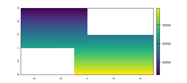
Crop and merge example.
r1 <- crop(r, ext(-50,0,0,30))
r2 <- crop(r, ext(-10,50,-20, 10))
m <- merge(r1, r2, filename="test.tif", overwrite=TRUE)
plot(m)
flip lets you flip the data (reverse order) in horizontal or
vertical direction – typically to correct for a ‘communication problem’
between different R packages or a misinterpreted file. rotate lets
you rotate longitude/latitude rasters that have longitudes from 0 to 360
degrees (often used by climatologists) to the standard -180 to 180
degrees system. With t you can rotate a SpatRaster object 90
degrees.
Overlay
app (short for “apply”) allows you to do a computation for a single
SpatRaster object by providing a function, e.g. sum.
The lapp (layer-apply) function can be used as an alternative to the
raster algebra discussed above.
Classify
You can use classify to replace ranges of values with single values,
or to substitute (replace) single values with other values.
r <- rast(ncol=3, nrow=2)
values(r) <- 1:ncell(r)
values(r)
##      lyr.1
## [1,]     1
## [2,]     2
## [3,]     3
## [4,]     4
## [5,]     5
## [6,]     6
Set all values above 4 to NA
s <- app(r, fun=function(x){ x[x < 4] <- NA; return(x)} )
as.matrix(s)
##      lyr.1
## [1,]    NA
## [2,]    NA
## [3,]    NA
## [4,]     4
## [5,]     5
## [6,]     6
Divide the first raster with two times the square root of the second raster and add five.
rs <- c(r, s)
w <- lapp(rs, fun=function(x, y){ x / (2 * sqrt(y)) + 5 } )
as.matrix(w)
##          lyr1
## [1,]       NA
## [2,]       NA
## [3,]       NA
## [4,] 6.000000
## [5,] 6.118034
## [6,] 6.224745
Remove from r all values that are NA in w.
u <- mask(r, w)
as.matrix(u)
##      lyr.1
## [1,]    NA
## [2,]    NA
## [3,]    NA
## [4,]     4
## [5,]     5
## [6,]     6
Identify the cell values in u that are the same as in s.
v <- u==s
as.matrix(v)
##      lyr.1
## [1,]    NA
## [2,]    NA
## [3,]    NA
## [4,]  TRUE
## [5,]  TRUE
## [6,]  TRUE
Replace NA values in w with values of r.
cvr <- cover(w, r)
as.matrix(w)
##          lyr1
## [1,]       NA
## [2,]       NA
## [3,]       NA
## [4,] 6.000000
## [5,] 6.118034
## [6,] 6.224745
Change value between 0 and 2 to 1, etc.
x <- classify(w, rbind(c(0,2,1),  c(2,5,2), c(4,10,3)))
as.matrix(x)
##      lyr1
## [1,]  NaN
## [2,]  NaN
## [3,]  NaN
## [4,]    3
## [5,]    3
## [6,]    3
Substitute 2 with 40 and 3 with 50.
y <- classify(x, cbind(id=c(2,3), v=c(40,50)))
as.matrix(y)
##      lyr1
## [1,]  NaN
## [2,]  NaN
## [3,]  NaN
## [4,]   50
## [5,]   50
## [6,]   50
Focal methods
The focal methods computate new values based on the values in a
neighborhood of cells around a focal cell, and putting the result in the
focal cell of the output SpatRaster. The neighborhood is a user-defined
matrix of weights and could approximate any shape by giving some cells
zero weight. It is possible to only computes new values for cells that
are NA in the input SpatRaster.
Distance
There are a number of distance related functions. For example, you can
compute the shortest distance to cells that are not NA, the shortest
distance to any point in a set of points, or the distance when following
grid cells that can be traversed (e.g. excluding water bodies).
direction computes the direction toward (or from) the nearest cell
that is not NA. adjacency determines which cells are adjacent to
other cells. See the gdistance package for more advanced distance
calculations (cost distance, resistance distance).
Spatial configuration
patches identifies groups of cells that are connected.
boundaries identifies edges, that is, transitions between cell
values. area computes the size of each grid cell (for unprojected
rasters), this may be useful to, e.g. compute the area covered by a
certain class on a longitude/latitude raster.
r <- rast(nrow=45, ncol=90)
values(r) <- round(runif(ncell(r))*3)
a <- cellSize(r)
zonal(a, r, "sum")
##   lyr.1         area
## 1     0 9.391452e+13
## 2     1 1.694339e+14
## 3     2 1.586069e+14
## 4     3 8.811029e+13
Predictions
The terra package has two functions to make model predictions to
(potentially very large) rasters. predict takes a multilayer raster
and a fitted model as arguments. Fitted models can be of various
classes, including glm, gam, and RandomForest. The function
interpolate is similar but is for models that use coordinates as
predictor variables, for example in Kriging and spline interpolation.
Vector to raster conversion
The terra package supports point, line, and polygon to raster conversion
with the rasterize function. For vector type data (points, lines,
polygons), SpatVector objects are used; but points can also be
represented by a two-column matrix (x and y).
Point to raster conversion is often done with the purpose to analyze the
point data. For example to count the number of distinct species
(represented by point observations) that occur in each raster cell.
rasterize takes a SpatRaster object to set the spatial extent
and resolution, and a function to determine how to summarize the points
(or an attribute of each point) by cell.
Polygon to raster conversion is typically done to create a
SpatRaster that can act as a mask, i.e. to set to NA a set of
cells of a SpatRaster object, or to summarize values on a raster by
zone. For example a country polygon is transferred to a raster that is
then used to set all the cells outside that country to NA; whereas
polygons representing administrative regions such as states can be
transferred to a raster to summarize raster values by region.
It is also possible to convert the values of a SpatRaster to points
or polygons, using as.points and as.polygons. Both functions
only return values for cells that are not NA.
Summarizing functions
When used with a SpatRaster object as first argument, normal summary
statistics functions such as min, max and mean return a
SpatRaster. You can use global if, instead, you want to obtain a
summary for all cells of a single SpatRaster object. You can use
freq to make a frequency table, or to count the number of cells with
a specified value. Use zonal to summarize a SpatRaster object
using zones (areas with the same integer number) defined in a
SpatRaster and crosstab to cross-tabulate two SpatRaster
objects.
r <- rast(ncol=36, nrow=18)
values(r) <- runif(ncell(r))
global(r, mean)
##            mean
## lyr.1 0.5179682
Zonal stats, below r has the cells we want to summarize, s
defines the zones, and the last argument is the function to summarize
the values of r for each zone in s.
s <- r
values(s) <- round(runif(ncell(r)) * 5)
zonal(r, s, 'mean')
##   lyr.1   lyr.1.1
## 1     0 0.5144431
## 2     1 0.5480089
## 3     2 0.5249257
## 4     3 0.5194031
## 5     4 0.4853966
## 6     5 0.5218401
Count cells
freq(s)
##   layer value count
## 1     1     0    54
## 2     1     1   102
## 3     1     2   139
## 4     1     3   148
## 5     1     4   133
## 6     1     5    72
freq(s, value=3)
##   layer value count
## 1     1     3   148
Cross-tabulate
ctb <- crosstab(c(r*3, s))
head(ctb)
##      lyr.1.1
## lyr.1  0  1  2  3  4  5
##     0  8 13 21 16 24 10
##     1 17 31 42 56 45 24
##     2 19 31 52 54 37 27
##     3 10 27 24 22 27 11
Helper functions
The cell number is an important concept in the terra package. Raster
data can be thought of as a matrix, but in a SpatRaster it is more
commonly treated as a vector. Cells are numbered from the upper left
cell to the upper right cell and then continuing on the left side of the
next row, and so on until the last cell at the lower right side of the
raster. There are several helper functions to determine the column or
row number from a cell and vice versa, and to determine the cell number
for x, y coordinates and vice versa.
r <- rast(ncol=36, nrow=18)
ncol(r)
## [1] 36
nrow(r)
## [1] 18
ncell(r)
## [1] 648
rowFromCell(r, 100)
## [1] 3
colFromCell(r, 100)
## [1] 28
cellFromRowCol(r,5,5)
## [1] 149
xyFromCell(r, 100)
##       x  y
## [1,] 95 65
cellFromXY(r, cbind(0,0))
## [1] 343
colFromX(r, 0)
## [1] 19
rowFromY(r, 0)
## [1] 10
Accessing cell values
Cell values can be accessed with several methods. Use values to get
all values or a subset such as a single row or a block (rectangle) of
cell values.
r <- rast(system.file("ex/elev.tif", package="terra"))
v <- values(r)
v[3075:3080, ]
## [1] 324 288 342 313 311 291
values(r, row=33, nrow=1, col=35, ncol=6)
##      elevation
## [1,]       324
## [2,]       288
## [3,]       342
## [4,]       313
## [5,]       311
## [6,]       291
You can also read values using cell numbers or coordinates (xy) using
the extract method.
cells <- cellFromRowCol(r, 33, 35:40)
cells
## [1] 3075 3076 3077 3078 3079 3080
r[cells]
##   elevation
## 1       324
## 2       288
## 3       342
## 4       313
## 5       311
## 6       291
xy <- xyFromCell(r, cells)
xy
##             x        y
## [1,] 6.029167 49.92083
## [2,] 6.037500 49.92083
## [3,] 6.045833 49.92083
## [4,] 6.054167 49.92083
## [5,] 6.062500 49.92083
## [6,] 6.070833 49.92083
extract(r, xy)
##   elevation
## 1       324
## 2       288
## 3       342
## 4       313
## 5       311
## 6       291
You can also extract values using SpatVector objects. The default
approach for extracting raster values with polygons is that a polygon
has to cover the center of a cell, for the cell to be included. However,
you can use argument weights=TRUE in which case you get, apart from
the cell values, the percentage of each cell that is covered by the
polygon, so that you can apply, e.g., a “50% area covered” threshold, or
compute an area-weighted average.
In the case of lines, any cell that is crossed by a line is included. For lines and points, a cell that is only ‘touched’ is included when it is below or to the right (or both) of the line segment/point (except for the bottom row and right-most column).
In addition, you can use standard R indexing to access values, or to
replace values (assign new values to cells) in a SpatRaster object.
If you replace a value in a SpatRaster object based on a file, the
connection to that file is lost (because it now is different from that
file). Setting raster values for very large files will be very slow with
this approach as each time a new (temporary) file, with all the values,
is written to disk. If you want to overwrite values in an existing file,
you can use update (with caution!)
r[cells]
##   elevation
## 1       324
## 2       288
## 3       342
## 4       313
## 5       311
## 6       291
r[1:4]
##   elevation
## 1        NA
## 2        NA
## 3        NA
## 4        NA
sources(r)
## [1] "C:/soft/R/R-4.5.3/library/terra/ex/elev.tif"
r[2:5] <- 10
r[1:4]
##   elevation
## 1        NA
## 2        10
## 3        10
## 4        10
sources(r)
## [1] ""
Note that in the above examples values are retrieved using cell numbers. That is, a raster is represented as a (one-dimensional) vector. Values can also be inspected using a (two-dimensional) matrix notation. As for R matrices, the first index represents the row number, the second the column number.
r[1:3]
##   elevation
## 1        NA
## 2        10
## 3        10
r[1,1:3]
##   elevation
## 1        NA
## 2        10
## 3        10
r[1, 1:5]
##   elevation
## 1        NA
## 2        10
## 3        10
## 4        10
## 5        10
r[1:5, 2]
##   elevation
## 1        10
## 2        NA
## 3        NA
## 4        NA
## 5        NA
r[1:3,1:3]
##   elevation
## 1        NA
## 2        10
## 3        10
## 4        NA
## 5        NA
## 6        NA
## 7        NA
## 8        NA
## 9        NA

# get a vector instead of a a matrix
r[1:3, 1:3, drop=TRUE]
##   elevation
## 1        NA
## 2        10
## 3        10
## 4        NA
## 5        NA
## 6        NA
## 7        NA
## 8        NA
## 9        NA

# or a raster like matrix
as.matrix(r, wide=TRUE)[1:3, 1:4]
##      [,1] [,2] [,3] [,4]
## [1,]   NA   10   10   10
## [2,]   NA   NA   NA   NA
## [3,]   NA   NA   NA   NA
Accessing values through this type of indexing should be avoided inside
functions as it is less efficient than accessing values via functions
like values.
Coercion to other classes
You can convert SpatRaster objects to Raster* objects defined in
the raster package.
r <- rast(ncol=36, nrow=18)
values(r) <- runif(ncell(r))
library(raster)
## Loading required package: sp
x <- raster(r)