Local regression
Regression models are typically “global”. That is, all date are used simultaneously to fit a single model. In some cases it can make sense to fit more flexible “local” models. Such models exist in a general regression framework (e.g. generalized additive models), where “local” refers to the values of the predictor values. In a spatial context local refers to location. Rather than fitting a single regression model, it is possible to fit several models, one for each location (out of possibly very many) locations. This technique is sometimes called “geographically weighted regression” (GWR). GWR is a data exploration technique that allows to understand changes in importance of different variables over space (which may indicate that the model used is mis-specified and can be improved).
There are two examples here. One short example with California precipitation data, and than a more elaborate example with house price data.
California precipitation
if (!require("rspat")) remotes::install_github('rspatial/rspat')
## Loading required package: rspat
## Loading required package: terra
## terra 1.9.21
library(rspat)
counties <- spat_data("counties")
p <- spat_data("precipitation")
head(p)
## ID NAME LAT LONG ALT JAN FEB MAR APR MAY JUN JUL
## 1 ID741 DEATH VALLEY 36.47 -116.87 -59 7.4 9.5 7.5 3.4 1.7 1.0 3.7
## 2 ID743 THERMAL/FAA AIRPORT 33.63 -116.17 -34 9.2 6.9 7.9 1.8 1.6 0.4 1.9
## 3 ID744 BRAWLEY 2SW 32.96 -115.55 -31 11.3 8.3 7.6 2.0 0.8 0.1 1.9
## 4 ID753 IMPERIAL/FAA AIRPORT 32.83 -115.57 -18 10.6 7.0 6.1 2.5 0.2 0.0 2.4
## 5 ID754 NILAND 33.28 -115.51 -18 9.0 8.0 9.0 3.0 0.0 1.0 8.0
## 6 ID758 EL CENTRO/NAF 32.82 -115.67 -13 9.8 1.6 3.7 3.0 0.4 0.0 3.0
## AUG SEP OCT NOV DEC
## 1 2.8 4.3 2.2 4.7 3.9
## 2 3.4 5.3 2.0 6.3 5.5
## 3 9.2 6.5 5.0 4.8 9.7
## 4 2.6 8.3 5.4 7.7 7.3
## 5 9.0 7.0 8.0 7.0 9.0
## 6 10.8 0.2 0.0 3.3 1.4
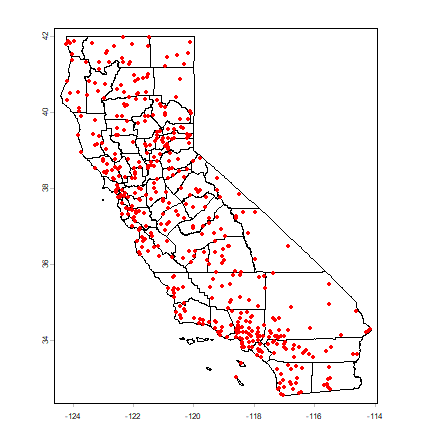
plot(counties)
points(p[,c("LONG", "LAT")], col="red", pch=20)
Compute annual average precipitation
p$pan <- rowSums(p[,6:17])
Global regression model
m <- lm(pan ~ ALT, data=p)
m
##
## Call:
## lm(formula = pan ~ ALT, data = p)
##
## Coefficients:
## (Intercept)          ALT
##      523.60         0.17
Create a SpatVector objects with a planar crs.
alb <- "+proj=aea +lat_1=34 +lat_2=40.5 +lat_0=0 +lon_0=-120 +x_0=0 +y_0=-4000000 +datum=WGS84 +units=m"
sp <- vect(p, c("LONG", "LAT"), crs="+proj=longlat +datum=WGS84")
spt <- project(sp, alb)
ctst <- project(counties, alb)
Get the optimal bandwidth
library( spgwr )
## Loading required package: sp
## Loading required package: spData
## To access larger datasets in this package, install the spDataLarge
## package with: `install.packages('spDataLarge',
## repos='https://nowosad.github.io/drat/', type='source')`
## NOTE: This package does not constitute approval of GWR
## as a method of spatial analysis; see example(gwr)
bw <- gwr.sel(pan ~ ALT, data=as.data.frame(spt), coords=geom(spt)[,c("x", "y")])
## Bandwidth: 526221.1 CV score: 64886883
## Bandwidth: 850593.6 CV score: 74209073
## Bandwidth: 325747.9 CV score: 54001118
## Bandwidth: 201848.6 CV score: 44611213
## Bandwidth: 125274.7 CV score: 35746320
## Bandwidth: 77949.39 CV score: 29181737
## Bandwidth: 48700.74 CV score: 22737197
## Bandwidth: 30624.09 CV score: 17457161
## Bandwidth: 19452.1 CV score: 15163436
## Bandwidth: 12547.43 CV score: 19452191
## Bandwidth: 22792.75 CV score: 15512988
## Bandwidth: 17052.67 CV score: 15709960
## Bandwidth: 20218.99 CV score: 15167438
## Bandwidth: 19767.99 CV score: 15156913
## Bandwidth: 19790.05 CV score: 15156906
## Bandwidth: 19781.39 CV score: 15156902
## Bandwidth: 19781.48 CV score: 15156902
## Bandwidth: 19781.47 CV score: 15156902
## Bandwidth: 19781.47 CV score: 15156902
## Bandwidth: 19781.47 CV score: 15156902
## Bandwidth: 19781.47 CV score: 15156902
bw
## [1] 19781.47
Create a regular set of points to estimate parameters for.
r <- rast(ctst, res=10000)
r <- rasterize(ctst, r)
newpts <- as.points(r)
Run the gwr function
g <- gwr(pan ~ ALT, data=as.data.frame(spt), coords=geom(spt)[,c("x", "y")], bandwidth=bw, fit.points=geom(newpts)[,c("x", "y")])
g
## Call:
## gwr(formula = pan ~ ALT, data = as.data.frame(spt), coords = geom(spt)[,
##     c("x", "y")], bandwidth = bw, fit.points = geom(newpts)[,
##     c("x", "y")])
## Kernel function: gwr.Gauss
## Fixed bandwidth: 19781.47
## Fit points: 4090
## Summary of GWR coefficient estimates at fit points:
##                     Min.     1st Qu.      Median     3rd Qu.      Max.
## X.Intercept. -846.314349   77.986477  328.579339  729.588989 3452.1972
## ALT            -3.961701    0.034149    0.201568    0.418716    4.6022
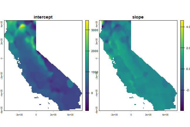
Link the results back to the raster
slope <- intercept <- r
slope[!is.na(slope)] <- g$SDF$ALT
intercept[!is.na(intercept)] <- g$SDF$'(Intercept)'
s <- c(intercept, slope)
names(s) <- c('intercept', 'slope')
plot(s)
California House Price Data
We will use house prices data from the 1990 census, taken from “Pace, R.K. and R. Barry, 1997. Sparse Spatial Autoregressions. Statistics and Probability Letters 33: 291-297.”
houses <- spat_data("houses1990.csv")
dim(houses)
## [1] 20640     9
head(houses)
##   houseValue income houseAge rooms bedrooms population households latitude
## 1     452600 8.3252       41   880      129        322        126    37.88
## 2     358500 8.3014       21  7099     1106       2401       1138    37.86
## 3     352100 7.2574       52  1467      190        496        177    37.85
## 4     341300 5.6431       52  1274      235        558        219    37.85
## 5     342200 3.8462       52  1627      280        565        259    37.85
## 6     269700 4.0368       52   919      213        413        193    37.85
##   longitude
## 1   -122.23
## 2   -122.22
## 3   -122.24
## 4   -122.25
## 5   -122.25
## 6   -122.25
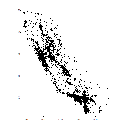
Each record represents a census “blockgroup”. The longitude and latitude of the centroids of each block group are available. We can use that to make a map and we can also use these to link the data to other spatial data. For example to get county-membership of each block group. To do that, let’s first turn this into a SpatialPointsDataFrame to find out to which county each point belongs.
hvect <- vect(houses, c("longitude", "latitude"))
## Warning: [vect] guessed crs
plot(hvect, cex=0.5, pch=1, axes=TRUE)
Now get the county boundaries and assign CRS of the houses data matches that of the counties (because they are both in longitude/latitude!).
crs(hvect) <- crs(counties)
Do a spatial query (points in polygon)
cnty <- extract(counties, hvect)
head(cnty)
##   id.y STATE COUNTY    NAME LSAD LSAD_TRANS
## 1    1    06    001 Alameda   06     County
## 2    2    06    001 Alameda   06     County
## 3    3    06    001 Alameda   06     County
## 4    4    06    001 Alameda   06     County
## 5    5    06    001 Alameda   06     County
## 6    6    06    001 Alameda   06     County
Summarize
We can summarize the data by county. First combine the extracted county data with the original data.
hd <- cbind(data.frame(houses), cnty)
Compute the population by county
totpop <- tapply(hd$population, hd$NAME, sum)
totpop
##         Alameda          Alpine          Amador           Butte       Calaveras
##         1241779            1113           30039          182120           31998
##          Colusa    Contra Costa       Del Norte       El Dorado          Fresno
##           16275          799017           16045          128624          662261
##           Glenn        Humboldt        Imperial            Inyo            Kern
##           24798          116418          108633           18281          528995
##           Kings            Lake          Lassen     Los Angeles          Madera
##           91842           50631           27214         8721937           88089
##           Marin        Mariposa       Mendocino          Merced           Modoc
##          204241           14302           75061          176457            9678
##            Mono        Monterey            Napa          Nevada          Orange
##            9956          342314          108030           78510         2340204
##          Placer          Plumas       Riverside      Sacramento      San Benito
##          170761           19739         1162787         1038540           36697
##  San Bernardino       San Diego   San Francisco     San Joaquin San Luis Obispo
##         1409740         2425153          683068          477184          203764
##       San Mateo   Santa Barbara     Santa Clara      Santa Cruz          Shasta
##          614816          335177         1486054          216732          147036
##          Sierra        Siskiyou          Solano          Sonoma      Stanislaus
##            3318           43531          337429          385296          370821
##          Sutter          Tehama         Trinity          Tulare        Tuolumne
##           63689           49625           13063          309073           48456
##         Ventura            Yolo            Yuba
##          649935          138799           58954
Income is harder because we have the median household income by blockgroup. But it can be approximated by first computing total income by blockgroup, summing that, and dividing that by the total number of households.
# total income
hd$suminc <- hd$income * hd$households
# now use aggregate (similar to tapply)
csum <- aggregate(hd[, c('suminc', 'households')], list(hd$NAME), sum)
# divide total income by number of housefholds
csum$income <- 10000 * csum$suminc / csum$households
# sort
csum <- csum[order(csum$income), ]
head(csum)
##     Group.1    suminc households   income
## 53  Trinity 11198.985       5156 21720.30
## 58     Yuba 43739.708      19882 21999.65
## 25    Modoc  8260.597       3711 22259.76
## 47 Siskiyou 38769.952      17302 22407.79
## 17     Lake 47612.899      20805 22885.32
## 11    Glenn 20497.683       8821 23237.37
tail(csum)
##         Group.1    suminc households   income
## 56      Ventura  994094.8     210418 47243.81
## 7  Contra Costa 1441734.6     299123 48198.72
## 30       Orange 3938638.1     800968 49173.48
## 43  Santa Clara 2621895.6     518634 50553.87
## 41    San Mateo 1169145.6     230674 50683.89
## 21        Marin  436808.4      85869 50869.17
Regression
Before we make a regression model, let’s first add some new variables that we might use, and then see if we can build a regression model with house price as dependent variable. The authors of the paper used a lot of log tranforms, so you can also try that.
hd$roomhead <- hd$rooms / hd$population
hd$bedroomhead <- hd$bedrooms / hd$population
hd$hhsize <- hd$population / hd$households
Ordinary least squares regression:
# OLS
m <- glm( houseValue ~ income + houseAge + roomhead + bedroomhead + population, data=hd)
summary(m)
##
## Call:
## glm(formula = houseValue ~ income + houseAge + roomhead + bedroomhead +
##     population, data = hd)
##
## Coefficients:
##               Estimate Std. Error t value Pr(>|t|)
## (Intercept) -6.508e+04  2.533e+03 -25.686  < 2e-16 ***
## income       5.179e+04  3.833e+02 135.092  < 2e-16 ***
## houseAge     1.832e+03  4.575e+01  40.039  < 2e-16 ***
## roomhead    -4.720e+04  1.489e+03 -31.688  < 2e-16 ***
## bedroomhead  2.648e+05  6.820e+03  38.823  < 2e-16 ***
## population   3.947e+00  5.081e-01   7.769 8.27e-15 ***
## ---
## Signif. codes:  0 '***' 0.001 '**' 0.01 '*' 0.05 '.' 0.1 ' ' 1
##
## (Dispersion parameter for gaussian family taken to be 6022427437)
##
##     Null deviance: 2.7483e+14  on 20639  degrees of freedom
## Residual deviance: 1.2427e+14  on 20634  degrees of freedom
## AIC: 523369
##
## Number of Fisher Scoring iterations: 2
coefficients(m)
##   (Intercept)        income      houseAge      roomhead   bedroomhead
## -65075.701407  51786.005862   1831.685266 -47198.908765 264766.186284
##    population
##      3.947461
Geographicaly Weighted Regression
By county
Of course we could make the model more complex, with e.g. squared income, and interactions. But let’s see if we can do Geographically Weighted regression. One approach could be to use counties.
First I remove records that were outside the county boundaries
hd2 <- hd[!is.na(hd$NAME), ]
Then I write a function to get what I want from the regression (the coefficients in this case)
regfun <- function(x)  {
  dat <- hd2[hd2$NAME == x, ]
  m <- glm(houseValue~income+houseAge+roomhead+bedroomhead+population, data=dat)
  coefficients(m)
}
And now run this for all counties using sapply:
countynames <- unique(hd2$NAME)
res <- sapply(countynames, regfun)
Plot of a single coefficient
dotchart(sort(res["income", ]), cex=0.65)
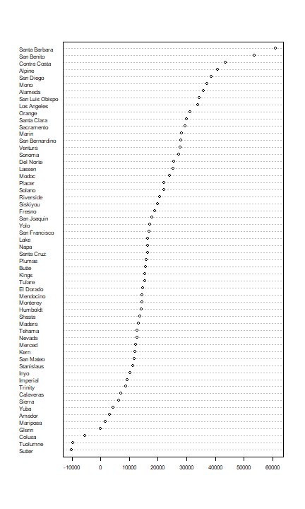
There clearly is variation in the coefficient (\(beta\)) for income. How does this look on a map?
First make a data.frame of the results
resdf <- data.frame(NAME=colnames(res), t(res))
head(resdf)
##                      NAME X.Intercept.    income  houseAge   roomhead
## Alameda           Alameda    -62373.62 35842.330  591.1001 24147.3182
## Contra Costa Contra Costa    -61759.84 43668.442  465.8897  -356.6085
## Alpine             Alpine    -77605.93 40850.588 5595.4113         NA
## Amador             Amador    120480.71  3234.519 -771.5857 37997.0069
## Butte               Butte     50935.36 15577.745 -380.5824  9078.9315
## Calaveras       Calaveras     91364.72  7126.668 -929.4065 16843.3456
##              bedroomhead population
## Alameda        129814.33  8.0570859
## Contra Costa   150662.89  0.8869663
## Alpine                NA         NA
## Amador        -194176.65  0.9971630
## Butte          -32272.68  5.7707597
## Calaveras      -78749.86  8.8865713
Fix the counties object. There are too many counties because of the presence of islands. I first aggregate (‘dissolve’ in GIS-speak’) the counties such that a single county becomes a single (multi-)polygon.
dim(counties)
## [1] 68  5
dcounties <- aggregate(counties[, "NAME"], "NAME")
dim(dcounties)
## [1] 58  2
Now we can merge this SpatVector with the data.frame with the regression results.
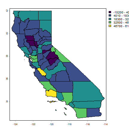
cnres <- merge(dcounties, resdf, by="NAME")
plot(cnres, "income")
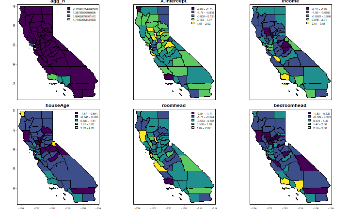
To show all parameters in a ‘conditioning plot’, we need to first scale the values to get similar ranges.
# a copy of the data
cnres2 <- cnres
# scale all variables, except the first one (county name)
values(cnres2) <- as.data.frame(scale(as.data.frame(cnres)[,-1]))
plot(cnres2, names(cnres2)[1:6], plg=list(x="topright"), mar=c(1,1,1,1))
Is this just random noise, or is there spatial autocorrelation?
lw <- adjacent(cnres2, pairs=FALSE)
autocor(cnres$income, lw)
## [1] 0.1565227
autocor(cnres$houseAge, lw)
## [1] -0.02057022
By grid cell
An alternative approach would be to compute a model for grid cells. Let’s use the ‘Teale Albers’ projection (often used when mapping the entire state of California).
TA <- "+proj=aea +lat_1=34 +lat_2=40.5 +lat_0=0 +lon_0=-120 +x_0=0 +y_0=-4000000 +datum=WGS84 +units=m"
countiesTA <- project(counties, TA)
Create a SpatRaster using the extent of the counties, and setting an arbitrary resolution of 50 by 50 km cells
r <- rast(countiesTA)
res(r) <- 50000
Get the xy coordinates for each raster cell:
xy <- xyFromCell(r, 1:ncell(r))
For each cell, we need to select a number of observations, let’s say within 50 km of the center of each cell (thus the data that are used in different cells overlap). And let’s require at least 50 observations to do a regression.
First transform the houses data to Teale-Albers
housesTA <- project(hvect, TA)
crds <- geom(housesTA)[, c("x", "y")]
Set up a new regression function.
regfun2 <- function(d)  {
 m <- glm(houseValue~income+houseAge+roomhead+bedroomhead+population, data=d)
 coefficients(m)
}
Run the model for al cells if there are at least 50 observations within a radius of 50 km.
res <- list()
for (i in 1:nrow(xy)) {
    d <- sqrt((xy[i,1]-crds[,1])^2 + (xy[i,2]-crds[,2])^2)
    j <- which(d < 50000)
    if (length(j) > 49) {
        d <- hd[j,]
        res[[i]] <- regfun2(d)
    } else {
        res[[i]] <- NA
    }
}
For each cell get the income coefficient:
inc <- sapply(res, function(x) x['income'])
Use these values in a SpatRaster
rinc <- setValues(r, inc)
plot(rinc)
plot(countiesTA, add=T)
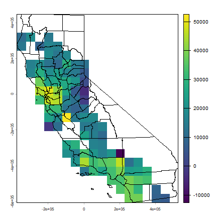
autocor(rinc)
##     lyr.1
## 0.4452912
So that was a lot of ‘home-brew-GWR’.
Question 1: Can you comment on weaknesses (and perhaps strengths) of the approaches I have shown?
spgwr package
Now use the spgwr package (and the the gwr function) to fit the
model. You can do this with all data, as long as you supply and argument
fit.points (to avoid estimating a model for each observation point.
You can use a raster similar to the one I used above (perhaps
disaggregate with a factor 2 first).
This is how you can get the points to use:
Create a SpatRaster with the correct extent
r <- rast(countiesTA)
Set to a desired resolution. I choose 25 km
res(r) <- 25000
I only want cells inside of CA, so I add some more steps.
ca <- rasterize(countiesTA, r)
Extract the coordinates that are not NA.
fitpoints <- crds(ca)
Now specify the model
gwr.model <- ______
gwr returns a list-like object that includes (as first element) a
SpatialPointsDataFrame that has the model coefficients. Plot these
and, after that, transfer them to a SpatRaster.
To extract the SpatialPointsDataFrame:
sp <- gwr.model$SDF
v <- vect(sp)
v
To reconnect these values to the raster structure (etc.)
cells <- cellFromXY(r, fitpoints)
dd <- as.matrix(data.frame(sp))
b <- rast(r, nl=ncol(dd))
b[cells] <- dd
names(b) <- colnames(dd)
plot(b)
Question 2: spgwr shows a remarkable startup message. What is that about?
Question 3: Briefly comment on the results and the differences (if any) with the two home-brew examples.