Spatial distribution models
This page shows how you can use the Random Forest algorithm to make spatial predictions. This approach is widely used, for example to classify remote sensing data into different land cover classes. But here our objective is to predict the entire range of a species based on a set of locations where it has been observed. As an example, we use the hominid species Imaginus magnapedum (also known under the vernacular names of “bigfoot” and “sasquatch”). This species is believed to occur in the United States, but it is so hard to find by scientists that its very existence is commonly denied by the mainstream media — despite the many reports on Twitter! For more information about this controversy, see the article by Lozier, Aniello and Hickerson: Predicting the distribution of Sasquatch in western North America: anything goes with ecological niche modelling.
We will use “citizen-science” data to find out:
What the complete range of the species might be.
How good (general) our model is by predicting the range of the Eastern sub-species, with data from the Western sub-species.
How climate change might affect its distribution.
In this context, this type of analysis is often referred to as ‘species distribution modeling’ or ‘ecological niche modeling’. Here is a more in-depth discussion of this technique.
First make sure we have the packages needed:
if (!require("rspat")) remotes::install_github("rspatial/rspat")
## Loading required package: rspat
## Loading required package: terra
## terra 1.9.21
if (!require("predicts")) install.packages("predicts")
## Loading required package: predicts
if (!require("geodata")) install.packages("geodata")
## Loading required package: geodata
Data
Observations
We get a data set of reported Bigfoot observations
library(terra)
library(rspat)
bf <- spat_data("bigfoot")
dim(bf)
## [1] 3092    3
head(bf)
##         lon      lat Class
## 1 -142.9000 61.50000     A
## 2 -132.7982 55.18720     A
## 3 -132.8202 55.20350     A
## 4 -141.5667 62.93750     A
## 5 -149.7853 61.05950     A
## 6 -141.3165 62.77335     A
It is always good to first plot the locations to see what we are dealing with.
plot(bf[,1:2], cex=0.5, col="red")
library(geodata)
wrld <- geodata::world(path=".")
bnds <- wrld[wrld$NAME_0 %in% c("Canada", "Mexico", "United States"), ]
lines(bnds)
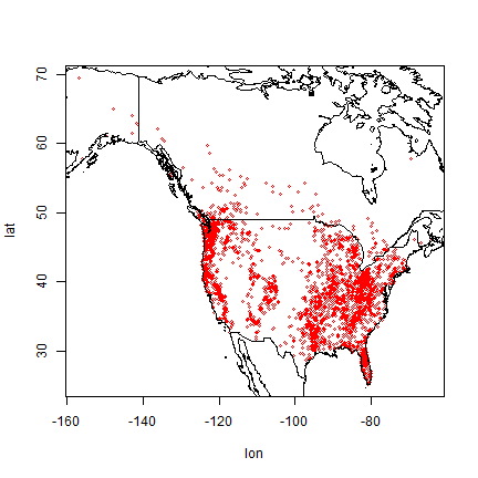
So the are in Canada and in the United States, but no reports from Mexico, so far.
Predictor variables
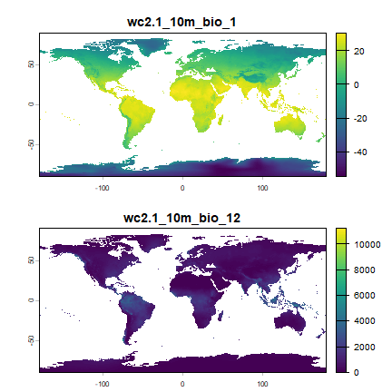
Here, as is common in species distribution modeling, we use climate data as predictor variables in our model. Specifically, we use “bioclimatic variables”, see: https://www.worldclim.org/data/bioclim.html. Here we used a spatial resolution of 10 minutes (one sixt of a degree). That is relatively coarse but it makes the download and processing faster.
wc <- geodata::worldclim_global("bio", res=10, ".")
plot(wc[[c(1, 12)]], nr=2)
Now extract climate data for the locations of our observations. In that way, we can find out what the climate conditions are that the species likes, apparently.
bfc <- extract(wc, bf[,1:2])
head(bfc, 3)
##   ID wc2.1_10m_bio_1 wc2.1_10m_bio_2 wc2.1_10m_bio_3 wc2.1_10m_bio_4
## 1  1       -1.832979       12.504708        28.95899       1152.4308
## 2  2        6.360650        5.865935        32.27475        462.5731
## 3  3        6.360650        5.865935        32.27475        462.5731
##   wc2.1_10m_bio_5 wc2.1_10m_bio_6 wc2.1_10m_bio_7 wc2.1_10m_bio_8
## 1        20.34075      -22.840000        43.18075        5.327750
## 2        16.65505       -1.519947        18.17500        3.964495
## 3        16.65505       -1.519947        18.17500        3.964495
##   wc2.1_10m_bio_9 wc2.1_10m_bio_10 wc2.1_10m_bio_11 wc2.1_10m_bio_12
## 1      -0.6887083         11.80792       -16.038542              991
## 2      10.4428196         12.28183         1.467686             3079
## 3      10.4428196         12.28183         1.467686             3079
##   wc2.1_10m_bio_13 wc2.1_10m_bio_14 wc2.1_10m_bio_15 wc2.1_10m_bio_16
## 1              120               42         31.32536              337
## 2              448              141         35.27518             1127
## 3              448              141         35.27518             1127
##   wc2.1_10m_bio_17 wc2.1_10m_bio_18 wc2.1_10m_bio_19
## 1              157              288              216
## 2              468              630              873
## 3              468              630              873
I remove the first column with the ID that we do not need.
bfc <- bfc[,-1]
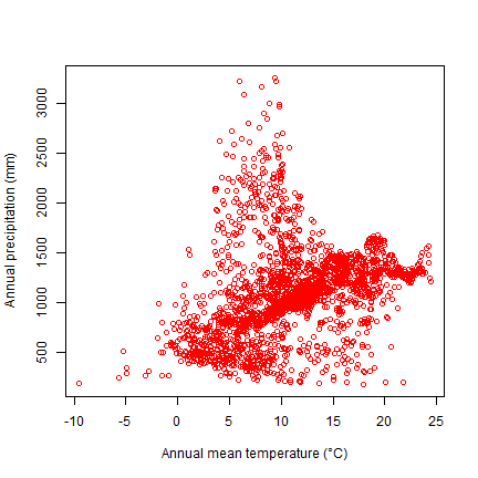
Now we can plot the species’ distribution in a part of the environmental space. Here is a plot of temperature vs rainfall of sites where Bigfoot was observed.
plot(bfc[ ,"wc2.1_10m_bio_1"], bfc[, "wc2.1_10m_bio_12"], col="red",
        xlab="Annual mean temperature (°C)", ylab="Annual precipitation (mm)")
Background data
Normally, one would build a model that would compare the values of the predictor variables at the locations where something was observed, with those values at the locations where it was not observed. But we do not have data from a systematic survey that determined presence and absence. We have presence-only data. (And, determining absence is not that simple. You blink and Bigfoot is gone!).
The common approach to deal with these type of data is to not model presence versus absence, but presence versus “background”. The “background” is the random (or maximum entropy) expectation; it is what you would get if the species had no preference for any of the predictor variables (or to other variables that are not in the model, but correlated with the predictor variables).
There is not much point in taking absence data from very far away (tropical Africa or Antarctica). Typically they are taken from more or less the entire study area for which we have presences data.
To do so, I first get the extent of all points
ext_bf <- ext(vect(bf[, 1:2])) + 1
## Warning: [vect] guessed crs
ext_bf
## SpatExtent : -157.75, -63.462699999999998, 24.140999999999998, 70.5 (xmin, xmax, ymin, ymax)
And then I take 5000 random samples (excluding NA cells) from
SpatExtent e, by using it as a “window” (blacking out all other
areas) on the climate SpatRaster.
set.seed(0)
window(wc) <- ext_bf
bg <- spatSample(wc, 5000, "random", na.rm=TRUE, xy=TRUE)
head(bg)
##           x        y wc2.1_10m_bio_1 wc2.1_10m_bio_2 wc2.1_10m_bio_3
## 1  -99.2500 66.75000     -13.2934895        7.870646        14.96619
## 2 -106.0833 42.08333       5.6722708       14.530958        36.82943
## 3 -111.9167 46.58333       6.7605939       14.135854        35.23372
## 4 -106.9167 54.75000       0.4086979       11.528605        24.43290
## 5 -118.2500 67.08333      -9.1363859        8.185354        16.34505
## 6 -111.2500 38.91667       8.4194584       15.997125        38.84047
##   wc2.1_10m_bio_4 wc2.1_10m_bio_5 wc2.1_10m_bio_6 wc2.1_10m_bio_7
## 1       1638.6833        15.42850       -37.16100        52.58950
## 2        894.3715        27.86600       -11.58875        39.45475
## 3        927.7927        28.14375       -11.97650        40.12025
## 4       1290.1088        22.55225       -24.63250        47.18475
## 5       1567.0846        17.46575       -32.61275        50.07850
## 6        904.0610        30.49050       -10.69625        41.18675
##   wc2.1_10m_bio_8 wc2.1_10m_bio_9 wc2.1_10m_bio_10 wc2.1_10m_bio_11
## 1        6.484917      -31.617332         7.518209        -31.76942
## 2        9.226916       -4.839750        17.168291         -4.83975
## 3       15.638333       -4.921750        18.186209         -4.92175
## 4       15.417084      -13.864500        15.417084        -16.31392
## 5        8.609292      -21.353209        10.573625        -27.49783
## 6       19.076958        3.179209        19.812834         -2.50475
##   wc2.1_10m_bio_12 wc2.1_10m_bio_13 wc2.1_10m_bio_14 wc2.1_10m_bio_15
## 1              171               33                4         70.29919
## 2              288               42               13         38.78144
## 3              293               48                9         53.40759
## 4              471               86               16         58.32499
## 5              223               43                7         61.21693
## 6              228               28               11         32.40370
##   wc2.1_10m_bio_16 wc2.1_10m_bio_17 wc2.1_10m_bio_18 wc2.1_10m_bio_19
## 1               90               13               78               13
## 2              112               41               90               41
## 3              129               35              115               35
## 4              220               53              220               56
## 5              108               27               93               29
## 6               83               40               72               44
Instead of using window you could also subset the climate data like
this wc <- crop(wc, ext_bf)
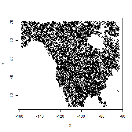
Above, with spatSample, I used the argument xy=TRUE to be able
to show were these points are from:
plot(bg[, c("x", "y")])
But we otherwise do not need them so I remove them again,
bg <- bg[, -c(1:2)]
We can now compare the climate of the presence and background points, for example, for temperature and rainfall
plot(bg[,1], bg[,12], xlab="Annual mean temperature (°C)",
          ylab="Annual precipitation (mm)", cex=.8)
points(bfc[,1], bfc[,12], col="red", cex=.6, pch="+")
legend("topleft", c("observed", "background"), col=c("red", "black"), pch=c("+", "o"), pt.cex=c(.6, .8))
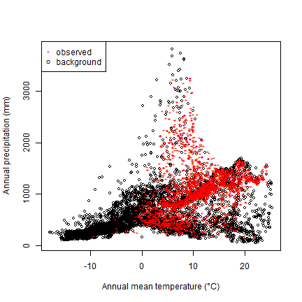
So we see that while Bigfoot is widespread, it is not common in cold areas, nor in hot and dry areas.
East vs West
I am first going to split the data into East and West. This is because I believe there are two sub-species (The Eastern Sasquatch is darker, less hairy, and has more pointy ears). I am principally interested in the western sub-species. Note how I use the original coordinates to subset the climate data. We can do this because they are in the same order.
#eastern points
bfe <- bfc[bf[,1] > -102, ]
#western points
bfw <- bfc[bf[,1] <= -102, ]
And now I combine the presence (“1”) with the background (“0”) data (I use the same background data for both subspecies)
dw <- rbind(cbind(pa=1, bfw), cbind(pa=0, bg))
de <- rbind(cbind(pa=1, bfe), cbind(pa=0, bg))
dw <- data.frame(dw)
de <- data.frame(na.omit(de))
dim(dw)
## [1] 6224   20
dim(de)
## [1] 6866   20
Fit a model
Now we have the data to fit a model. Let’s first look at a Classification and Regression Trees (CART) model.
CART
library(rpart)
cart <- rpart(pa~., data=dw)
The “complexity parameter” can be used as a stopping parameter to avoid overfitting.
printcp(cart)
##
## Regression tree:
## rpart(formula = pa ~ ., data = dw)
##
## Variables actually used in tree construction:
## [1] wc2.1_10m_bio_10 wc2.1_10m_bio_12 wc2.1_10m_bio_14 wc2.1_10m_bio_18
## [5] wc2.1_10m_bio_19 wc2.1_10m_bio_3  wc2.1_10m_bio_4
##
## Root node error: 983.29/6224 = 0.15798
##
## n= 6224
##
##         CP nsplit rel error  xerror     xstd
## 1 0.322797      0   1.00000 1.00019 0.019351
## 2 0.080521      1   0.67720 0.68771 0.019687
## 3 0.073325      2   0.59668 0.59759 0.015480
## 4 0.068645      3   0.52336 0.52163 0.015231
## 5 0.027920      4   0.45471 0.47026 0.014758
## 6 0.014907      5   0.42679 0.44778 0.015136
## 7 0.010869      6   0.41188 0.44082 0.015406
## 8 0.010197      7   0.40102 0.43500 0.015330
## 9 0.010000      8   0.39082 0.43197 0.015319
plotcp(cart)
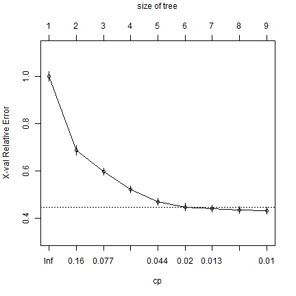
Fit the model again, with fewer splits
cart <- rpart(pa~., data=dw, cp=0.02)
And here is the tree
library(rpart.plot)
rpart.plot(cart, uniform=TRUE, main="Regression Tree")
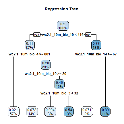
Question 1: What are the environmental conditions that Bigfoot appears to enjoy most?
And now we can use the model to show how attractive the climate is for this species.
x <- predict(wc, cart)
x <- mask(x, wc[[1]])
x <- round(x, 2)
plot(x, type="class", plg=list(x="bottomleft"))
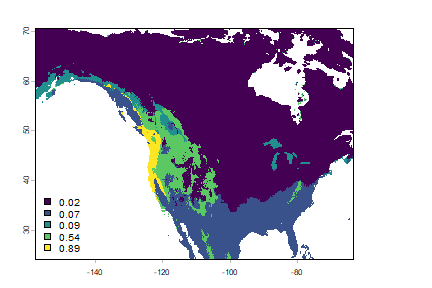
Notice that there are six values, because the regression tree has six leaves.
Random Forest
CART gives us a nice result to look at that can be easily interpreted (as you just illustrated with your answer to Question 1). But the approach suffers from high variance (meaning that the model tends to be over-fit, it is different each time a somewhat different datasets are used); and the quality of its predictions suffers from that. Random Forest does not have that problem as much. Above, with CART, we use regression, let’s do both regression and classification here.
But first I set some points aside for validation (normally we would do k-fold cross-validation, but we keep it simple here).
set.seed(123)
i <- sample(nrow(dw), 0.2 * nrow(dw))
test <- dw[i,]
train <- dw[-i,]
First we do classification, by making a categorical variable for presence/background.
fpa <- as.factor(train[, 'pa'])
Now fit the RandomForest model
library(randomForest)
## randomForest 4.7-1.2
## Type rfNews() to see new features/changes/bug fixes.
crf <- randomForest(train[, 2:ncol(train)], fpa)
crf
##
## Call:
##  randomForest(x = train[, 2:ncol(train)], y = fpa)
##                Type of random forest: classification
##                      Number of trees: 500
## No. of variables tried at each split: 4
##
##         OOB estimate of  error rate: 7.19%
## Confusion matrix:
##      0   1 class.error
## 0 3832 165  0.04128096
## 1  193 790  0.19633774
The Out-Of-Bag error rate is very small.
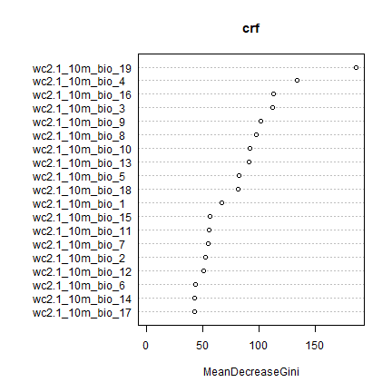
The variable importance plot shows which variables are most important in fitting the model. This is computed by randomizing each variable one by one, and then evaluating the decline in model prediction.
varImpPlot(crf)
Now we use regression, rather than classification. First we tune a parameter.
trf <- tuneRF(train[, 2:ncol(train)], train[, "pa"])
## Warning in randomForest.default(x, y, mtry = mtryStart, ntree = ntreeTry, : The
## response has five or fewer unique values.  Are you sure you want to do
## regression?
## mtry = 6  OOB error = 0.05594974
## Searching left ...
## Warning in randomForest.default(x, y, mtry = mtryCur, ntree = ntreeTry, : The
## response has five or fewer unique values.  Are you sure you want to do
## regression?
## mtry = 3     OOB error = 0.05612125
## -0.003065481 0.05
## Searching right ...
## Warning in randomForest.default(x, y, mtry = mtryCur, ntree = ntreeTry, : The
## response has five or fewer unique values.  Are you sure you want to do
## regression?
## mtry = 12    OOB error = 0.05485775
## 0.01951734 0.05
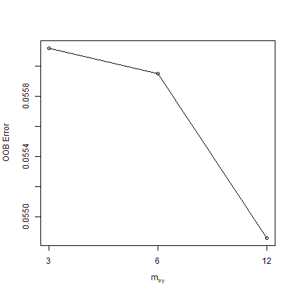
trf
##    mtry   OOBError
## 3     3 0.05612125
## 6     6 0.05594974
## 12   12 0.05485775
mt <- trf[which.min(trf[,2]), 1]
mt
## [1] 12
Question 2: What did tuneRF help us find? What does the values of mt represent?
rrf <- randomForest(train[, 2:ncol(train)], train[, "pa"], mtry=mt, ntree=250)
## Warning in randomForest.default(train[, 2:ncol(train)], train[, "pa"], mtry =
## mt, : The response has five or fewer unique values.  Are you sure you want to
## do regression?
rrf
##
## Call:
##  randomForest(x = train[, 2:ncol(train)], y = train[, "pa"], ntree = 250,      mtry = mt)
##                Type of random forest: regression
##                      Number of trees: 250
## No. of variables tried at each split: 12
##
##           Mean of squared residuals: 0.05421534
##                     % Var explained: 65.78
plot(rrf)
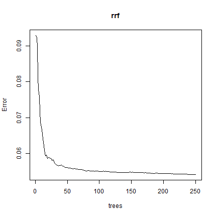
Question 3: What does ``plot(rrf)`` show us?
Predict
We can use the model to make predictions to any other place for which we have values for the predictor variables. Our climate data is global so we could find suitable areas for Bigfoot in Australia, but let’s stick to North America for now.
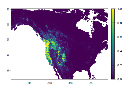
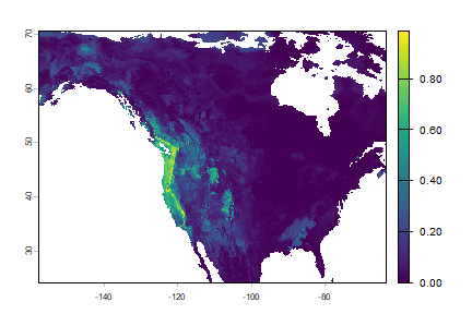
Regression
rp <- predict(wc, rrf, na.rm=TRUE)
plot(rp)
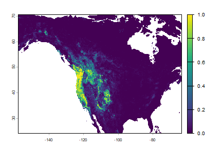
Note that the regression predictions are well-behaved, in the sense that they are between 0 and 1. However, they are continuous within that range, and if you wanted presence/absence, you would need a threshold. To get the optimal threshold, you would normally have a hold out data set, but here I use the training data for simplicity.
library(predicts)
eva <- pa_evaluate(predict(rrf, test[test$pa==1, ]), predict(rrf, test[test$pa==0, ]))
eva
## @stats
##    np   na prevalence   auc cor pcor   ODP
## 1 241 1003      0.194 0.965 0.8    0 0.806
##
## @thresholds
##   max_kappa max_spec_sens no_omission equal_prevalence equal_sens_spec
## 1     0.447         0.322       0.004            0.195           0.217
##
## @tr_stats
##     treshold kappa  CCR  TPR  TNR  FPR  FNR  PPP  NPP  MCR  OR
## 1          0     0 0.19    1    0    1    0 0.19  NaN 0.81 NaN
## 2          0  0.25 0.56    1 0.46 0.54    0 0.31    1 0.44 Inf
## 3          0  0.25 0.56    1 0.46 0.54    0 0.31    1 0.44 Inf
## 4        ...   ...  ...  ...  ...  ...  ...  ...  ...  ... ...
## 594        1  0.05 0.81 0.03    1    0 0.97    1 0.81 0.19 Inf
## 595        1  0.05 0.81 0.03    1    0 0.97    1 0.81 0.19 Inf
## 596        1     0 0.81    0    1    0    1  NaN 0.81 0.19 NaN
We can make a ROC plot
plot(eva, "ROC")
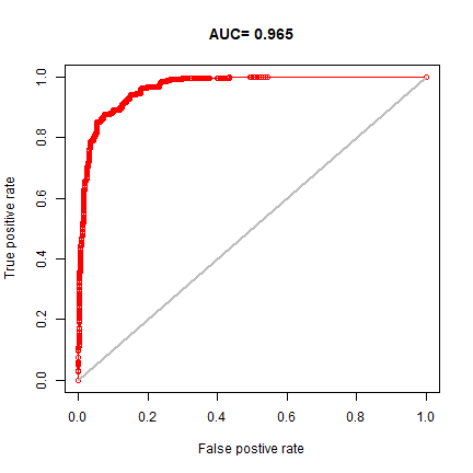
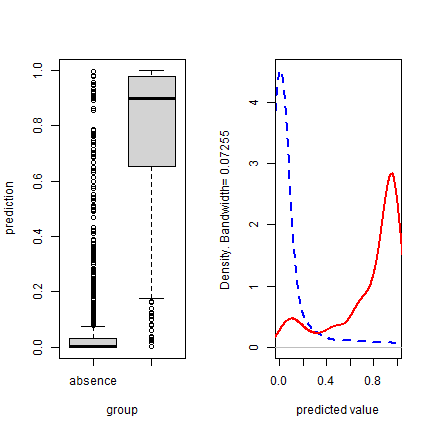
This suggests that the model is (very near) perfect in disinguising presence from background points. This is perhaps better illustrated with these plots:
par(mfrow=c(1,2))
plot(eva, "boxplot")
plot(eva, "density")
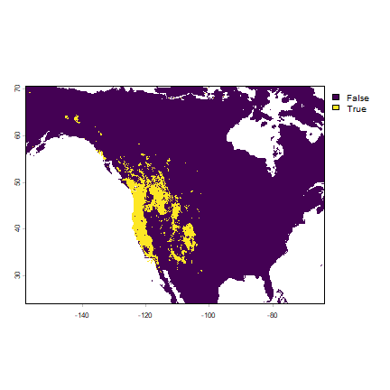
To get a good threshold to determine presence/absence and plot the prediction, we can use the “max specificity + sensitivity” threshold.
tr <- eva@thresholds
tr
##   max_kappa max_spec_sens no_omission equal_prevalence equal_sens_spec
## 1 0.4469667     0.3219856  0.00425973        0.1952333       0.2167239
plot(rp > tr$max_spec_sens)
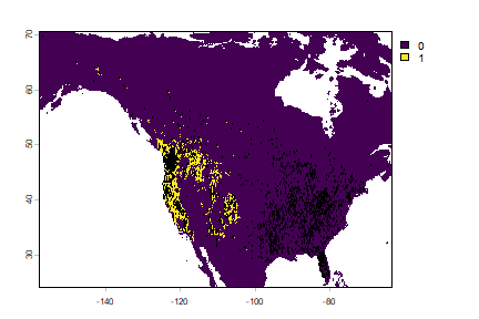
Classification
We can also use the classification Random Forest model to make a prediction.
rc <- predict(wc, crf, na.rm=TRUE)
plot(rc)
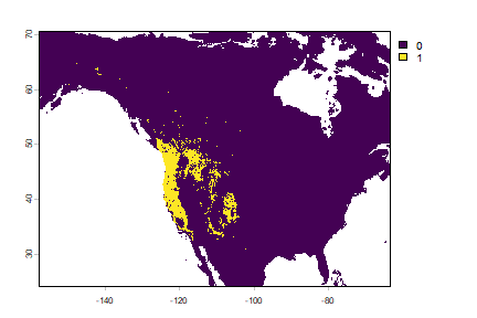
They are different because the classification used a threshold of 0.5, which is not necessarily appropriate.
You can get probabilities for the classes (in this case there are 2 classes, presence and absence, and I only plot presence)
rc2 <- predict(wc, crf, type="prob", na.rm=TRUE)
plot(rc2, 2)
Extrapolation
Now, let’s see if our model is general enough to predict the distribution of the Eastern species.
eva2 <- pa_evaluate(predict(rrf, de[de$pa==1, ]), predict(rrf, de[de$pa==0, ]))
eva2
## @stats
##     np   na prevalence   auc    cor pcor   ODP
## 1 1866 5000      0.272 0.561 -0.137    0 0.728
##
## @thresholds
##   max_kappa max_spec_sens no_omission equal_prevalence equal_sens_spec
## 1     0.001         0.001           0            0.271           0.001
##
## @tr_stats
##     treshold kappa  CCR  TPR TNR FPR  FNR  PPP  NPP  MCR   OR
## 1          0     0 0.27    1   0   1    0 0.27  NaN 0.73  NaN
## 2          0  0.02 0.51 0.53 0.5 0.5 0.47 0.28 0.74 0.49 1.12
## 3          0  0.02 0.51 0.53 0.5 0.5 0.47 0.28 0.74 0.49 1.12
## 4        ...   ...  ...  ... ... ...  ...  ...  ...  ...  ...
## 522     0.99     0 0.73    0   1   0    1    0 0.73 0.27    0
## 523     0.99     0 0.73    0   1   0    1  NaN 0.73 0.27  NaN
## 524     0.99     0 0.73    0   1   0    1  NaN 0.73 0.27  NaN
par(mfrow=c(1,2))
plot(eva2, "ROC")
plot(eva2, "boxplot")
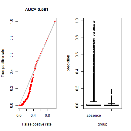
By this measure, it is a terrible model – as we already saw on the map. So our model is really good in predicting the range of the West, but it cannot extrapolate at all to the East.
plot(rc)
points(bf[,1:2], cex=.25)
Question 4: Why would it be that the model does not extrapolate well?
An important question in the biogeography of the Bigfoot would be if it can survive in other parts of the world (it has been spotted trying to get on commerical flights leaving North America).
Let’s see.
window(wc) <- NULL
pm <- predict(wc, rrf, na.rm=TRUE)
plot(pm)
lines(wrld)
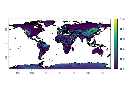
Question 5: What are some countries that should consider Bigfoot as a potential invasive species?
Climate change
We can also estimate range shifts due to climate change. We can use the same model, but now extrapolate in time (and space).
fut <- cmip6_world("CNRM-CM6-1", "585", "2061-2080", var="bio", res=10, path=".")
names(fut)
##  [1] "bio01" "bio02" "bio03" "bio04" "bio05" "bio06" "bio07" "bio08" "bio09"
## [10] "bio10" "bio11" "bio12" "bio13" "bio14" "bio15" "bio16" "bio17" "bio18"
## [19] "bio19"
names(wc)
##  [1] "wc2.1_10m_bio_1"  "wc2.1_10m_bio_2"  "wc2.1_10m_bio_3"  "wc2.1_10m_bio_4"
##  [5] "wc2.1_10m_bio_5"  "wc2.1_10m_bio_6"  "wc2.1_10m_bio_7"  "wc2.1_10m_bio_8"
##  [9] "wc2.1_10m_bio_9"  "wc2.1_10m_bio_10" "wc2.1_10m_bio_11" "wc2.1_10m_bio_12"
## [13] "wc2.1_10m_bio_13" "wc2.1_10m_bio_14" "wc2.1_10m_bio_15" "wc2.1_10m_bio_16"
## [17] "wc2.1_10m_bio_17" "wc2.1_10m_bio_18" "wc2.1_10m_bio_19"
names(fut) <- names(wc)
window(fut) <- ext_bf
pfut <- predict(fut, rrf, na.rm=TRUE)
plot(pfut)
Question 6: Make a map to show where conditions are improving for western bigfoot, and where they are not. Is the species headed toward extinction?
Further reading
More on Species distribution modeling with R.