Maps
You can make a map with plot(x), were x is a SpatRaster or a
SpatVector. You can add additional spatial data or text with
functions such as points, lines, text
You can zoom in using zoom(x) and clicking on the map twice (to
indicate where to zoom to). Or use sel(x) to save a spatial subset
to a new object. With click(x) it is possible to interactively query
a SpatRaster by clicking once or several times on a map plot.
SpatVector
Example data
library(terra)
## terra 1.9.21
p <- vect(system.file("ex/lux.shp", package="terra"))
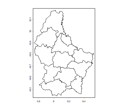
If you plot a SpatVector without further arguments, you get black
points, lines or polygons, and no legend.
plot(p)
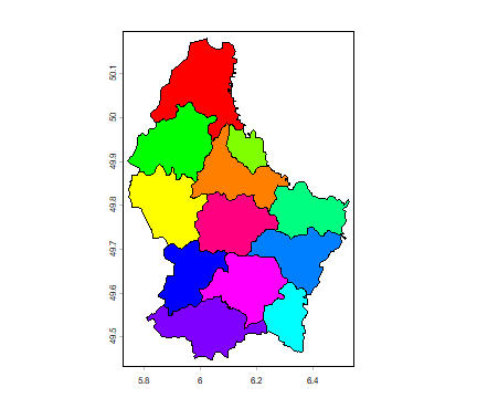
You can add colors like this
n <- nrow(p)
plot(p, col=rainbow(n))
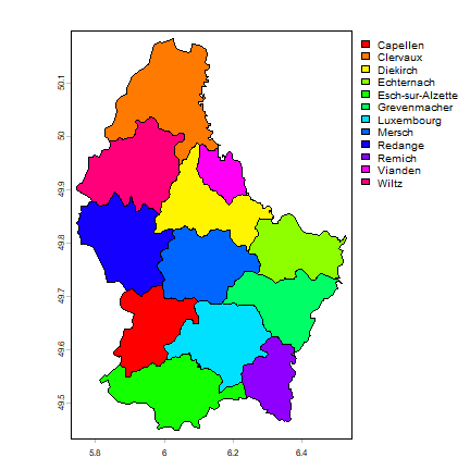
But if you want colors it is probably easiest to use an attribute.
plot(p, "NAME_2", col=rainbow(25))
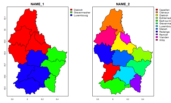
You can request maps for multiple variables
plot(p, c("NAME_1", "NAME_2"), col=rainbow(25))
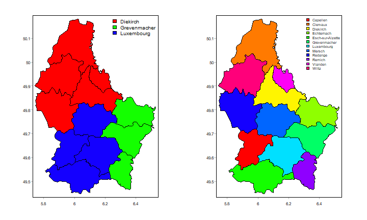
Below we also make two maps, but do it “by hand”. We adjust the spacing, and put the legends inside the map area, and use non-rotated text for the vertical axis.
par(mfrow=c(1,2))
m <- c(3.1, 3.1, 2.1, 2.1)
plot(p, "NAME_1", col=rainbow(25), mar=m, plg=list(x="topright"), pax=list(las=1))
plot(p, "NAME_2", col=rainbow(25), mar=m, plg=list(x="topright", cex=.75), pax=list(las=1))
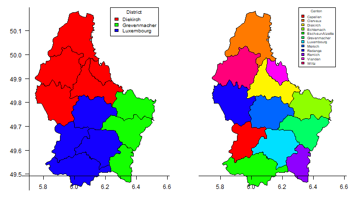
More costumization. Choose the axes to draw, at a label and a box to the legend.
par(mfrow=c(1,2))
m <- c(3.1, 3.1, 1.1, 1.1)
plot(p, "NAME_1", col=rainbow(25), mar=m, plg=list(x="topright", title="District", bty = "o"), main="", axes=FALSE)
axis(1, at=c(5,7)); axis(1)
axis(2, at=c(49,51)); axis(2, las=1)
plot(p, "NAME_2", col=rainbow(25), mar=m, plg=list(x="topright", cex=.75, title="Canton", bty = "o"), main="", axes=FALSE)
axis(1, at=c(5, 7)); axis(1)
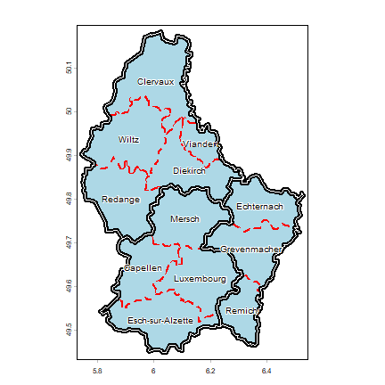
We can combine multiple SpatVectors using lines and points to
draw on top of what we plotted first.
d <- aggregate(p, "NAME_1")
plot(p, col="light blue", lty=2, border="red", lwd=2)
lines(d, lwd=5)
lines(d, col="white", lwd=1)
text(p, "NAME_2", cex=.8, halo=TRUE)
The rasterVis package provides a lot of very nice plotting options
as well.
SpatRaster
Example data
f <- system.file("ex/elev.tif", package="terra")
r <- rast(f)
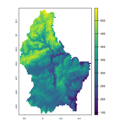
The default display of a single layer SpatRaster depends on the data type, but there will always be a legend.
plot(r)
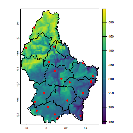
After plotting a SpatRaster you can add vector type spatial data
(points, lines, polygons). You can do this with functions points,
lines, polys or plot(object, add=TRUE).
plot(r)
lines(p, lwd=2)
set.seed(12)
xy <- spatSample(r, 20, "random", na.rm=TRUE, xy=TRUE)
points(xy, pch=20, col="red", cex=2)
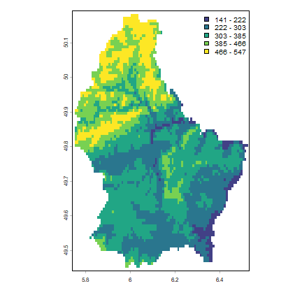
Or use a different legend type
m <- c(3.1, 3.1, 1.1, 1.1)
plot(r, type="interval", plg=list(x="topright"), mar=m)
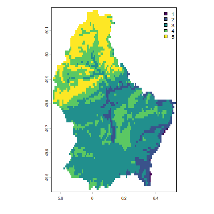
If there are only a few values, the default is to show “classes”
rr <- round(r/100)
plot(rr, plg=list(x="topright"), mar=m)
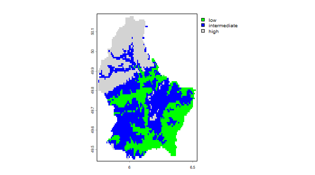
If the raster is categorical you get the category labels in the legend.
Make a categorical (factor) raster
x <- classify(r, c(140, 300, 400, 550))
levels(x) <- data.frame(id=0:2, elevation=c("low", "intermediate", "high"))
is.factor(x)
## [1] TRUE
x
## class       : SpatRaster
## size        : 90, 95, 1  (nrow, ncol, nlyr)
## resolution  : 0.008333333, 0.008333333  (x, y)
## extent      : 5.741667, 6.533333, 49.44167, 50.19167  (xmin, xmax, ymin, ymax)
## coord. ref. : lon/lat WGS 84 (EPSG:4326)
## source(s)   : memory
## varname     : elev
## name        : elevation
## min value   :         0
## max value   :         2
plot(x, col=c("green", "blue", "light gray"))
When plot is used with a multi-layer object, all layers are plotted (up to 16), unless the layers desired are indicated with an additional argument.
library(terra)
b <- rast(system.file("ex/logo.tif", package="terra"))
plot(b)

r <- rast(p, res=0.01 )
values(r) <- 1:ncell(r)
r <- mask(r, p)
In this case, it makes sense to combine the three layers into a single image, by assigning individual layers to one of the three color channels (red, green and blue):
plotRGB(b, r=1, g=2, b=3)

You can also use a number of other plotting functions with SpatRasters,
including hist, persp, contour}, and density. See the
help files for more info.
The rasterVis and tmap packages provides a lot of very nice
mapping options as well.
Basemaps
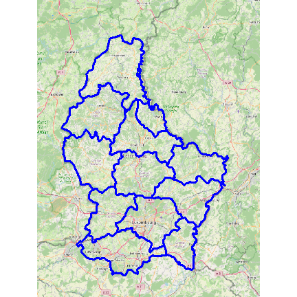
You can get many different base-maps with the maptiles package. Reading the data again.
library(terra)
f <- system.file("ex/lux.shp", package="terra")
p <- vect(f)
library(maptiles)
bg <- get_tiles(ext(p))
plotRGB(bg)
lines(p, col="blue", lwd=3)