Vector data manipulation
This chapter illustrates some ways in which we can manipulate vector data. We start with an example SpatVector that we read from a shapefile.
library(terra)
## terra 1.9.21
f <- system.file("ex/lux.shp", package="terra")
p <- vect(f)
p
## class       : SpatVector
## geometry    : polygons
## dimensions  : 12, 6  (geometries, attributes)
## extent      : 5.74414, 6.528252, 49.44781, 50.18162  (xmin, xmax, ymin, ymax)
## source      : lux.shp
## coord. ref. : lon/lat WGS 84 (EPSG:4326)
## names       :  ID_1   NAME_1  ID_2   NAME_2  AREA   POP
## type        : <num>    <chr> <num>    <chr> <num> <num>
## values      :     1 Diekirch     1 Clervaux   312 18081
##                   1 Diekirch     2 Diekirch   218 32543
##                   1 Diekirch     3  Redange   259 18664
##               ...
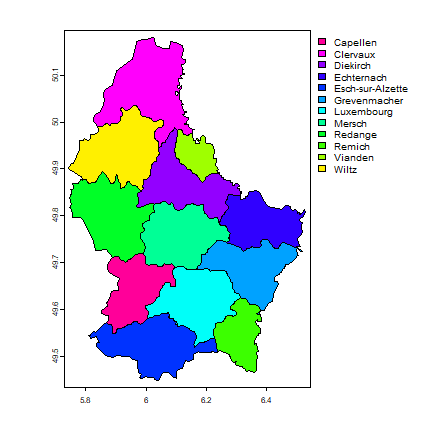
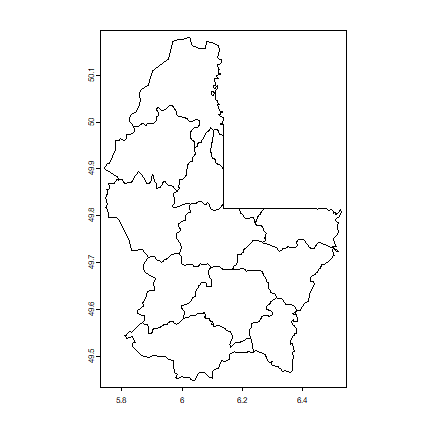
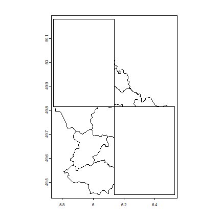
We can plot these data in many ways. For example:
plot(p, "NAME_2")
Basics
Geometry and attributes
To extract the attributes (data.frame) from a SpatVector, use:
d <- as.data.frame(p)
head(d)
##   ID_1       NAME_1 ID_2     NAME_2 AREA   POP
## 1    1     Diekirch    1   Clervaux  312 18081
## 2    1     Diekirch    2   Diekirch  218 32543
## 3    1     Diekirch    3    Redange  259 18664
## 4    1     Diekirch    4    Vianden   76  5163
## 5    1     Diekirch    5      Wiltz  263 16735
## 6    2 Grevenmacher    6 Echternach  188 18899
You can also extract the geometry as a a matrix (this is rarely needed).
g <- geom(p)
head(g)
##      geom part        x        y hole
## [1,]    1    1 6.026519 50.17767    0
## [2,]    1    1 6.031361 50.16563    0
## [3,]    1    1 6.035646 50.16410    0
## [4,]    1    1 6.042747 50.16157    0
## [5,]    1    1 6.043894 50.16116    0
## [6,]    1    1 6.048243 50.16008    0
Or as “well-known-text”
g <- geom(p, wkt=TRUE)
substr(g, 1, 50)
##  [1] "POLYGON ((6.0265188199999997 50.1776695300000029, "
##  [2] "POLYGON ((6.1783676099999996 49.8768234300000017, "
##  [3] "POLYGON ((5.8813781699999996 49.8701477099999977, "
##  [4] "POLYGON ((6.1313085599999999 49.9725646999999995, "
##  [5] "POLYGON ((5.9779286400000000 50.0260162399999970, "
##  [6] "POLYGON ((6.3855319000000001 49.8370285000000024, "
##  [7] "POLYGON ((6.3166646999999996 49.6233749399999979, "
##  [8] "POLYGON ((6.4251575499999998 49.7316436799999977, "
##  [9] "POLYGON ((5.9983120000000003 49.6999244699999991, "
## [10] "POLYGON ((6.0394744899999999 49.4482612600000024, "
## [11] "POLYGON ((6.1559634200000000 49.6850471500000026, "
## [12] "POLYGON ((6.0679822000000003 49.8284645100000034, "
Variables
You can extract a variable as you would do with a data.frame.
p$NAME_2
##  [1] "Clervaux"         "Diekirch"         "Redange"          "Vianden"
##  [5] "Wiltz"            "Echternach"       "Remich"           "Grevenmacher"
##  [9] "Capellen"         "Esch-sur-Alzette" "Luxembourg"       "Mersch"
To sub-set a SpatVector to one or more variables you can use the notation below. Note how this is different from the above example. Above a vector of values is returned. With the approach below you get a new SpatVector with only one variable.
p[, "NAME_2"]
## class       : SpatVector
## geometry    : polygons
## dimensions  : 12, 1  (geometries, attributes)
## extent      : 5.74414, 6.528252, 49.44781, 50.18162  (xmin, xmax, ymin, ymax)
## source      : lux.shp
## coord. ref. : lon/lat WGS 84 (EPSG:4326)
## names       :   NAME_2
## type        :    <chr>
## values      : Clervaux
##               Diekirch
##                Redange
##               ...
You can add a new variable to a SpatVector just as if it were a
data.frame.
set.seed(0)
p$lets <- sample(letters, nrow(p))
p
## class       : SpatVector
## geometry    : polygons
## dimensions  : 12, 7  (geometries, attributes)
## extent      : 5.74414, 6.528252, 49.44781, 50.18162  (xmin, xmax, ymin, ymax)
## source      : lux.shp
## coord. ref. : lon/lat WGS 84 (EPSG:4326)
## names       :  ID_1   NAME_1  ID_2   NAME_2  AREA   POP  lets
## type        : <num>    <chr> <num>    <chr> <num> <num> <chr>
## values      :     1 Diekirch     1 Clervaux   312 18081     n
##                   1 Diekirch     2 Diekirch   218 32543     y
##                   1 Diekirch     3  Redange   259 18664     d
##               ...
Note that to get the number of geometries of SpatVector p, you can
use nrow(p), or size(p). You can also do perim(p) to get the
“length” of the spatial objects (zero for points, the length of the
lines, or the perimeter of the polygons).
perim(p)
##  [1] 117100.12  93477.28  84502.45  44919.14  85032.61  74708.05  57991.42
##  [8]  81203.93  74443.82  95564.74  80618.76  70810.67
Assigning a new value to an existing variable.
p$lets <- sample(LETTERS, nrow(p))
head(p)
##   ID_1       NAME_1 ID_2     NAME_2 AREA   POP lets
## 1    1     Diekirch    1   Clervaux  312 18081    J
## 2    1     Diekirch    2   Diekirch  218 32543    V
## 3    1     Diekirch    3    Redange  259 18664    N
## 4    1     Diekirch    4    Vianden   76  5163    Z
## 5    1     Diekirch    5      Wiltz  263 16735    G
## 6    2 Grevenmacher    6 Echternach  188 18899    I
To get rid of a variable, set it to NULL.
p$lets <- NULL
Merge
You can assign an attributes table (data.frame) to a SpatVector with
values<-. To add attributes to a SpatVector that already has
attributes use merge (or cbind if you know the order of the
records is the same).
dfr <- data.frame(District=p$NAME_1, Canton=p$NAME_2, Value=round(runif(length(p), 100, 1000)))
dfr <- dfr[order(dfr$Canton), ]
pm <- merge(p, dfr, by.x=c('NAME_1', 'NAME_2'), by.y=c('District', 'Canton'))
pm
## class       : SpatVector
## geometry    : polygons
## dimensions  : 12, 7  (geometries, attributes)
## extent      : 5.74414, 6.528252, 49.44781, 50.18162  (xmin, xmax, ymin, ymax)
## coord. ref. : lon/lat WGS 84 (EPSG:4326)
## names       :   NAME_1   NAME_2  ID_1  ID_2  AREA   POP Value
## type        :    <chr>    <chr> <num> <num> <num> <num> <num>
## values      : Diekirch Clervaux     1     1   312 18081   406
##               Diekirch Diekirch     1     2   218 32543   534
##               Diekirch  Redange     1     3   259 18664   640
##               ...
head(pm)
##         NAME_1     NAME_2 ID_1 ID_2 AREA   POP Value
## 1     Diekirch   Clervaux    1    1  312 18081   406
## 2     Diekirch   Diekirch    1    2  218 32543   534
## 3     Diekirch    Redange    1    3  259 18664   640
## 4     Diekirch    Vianden    1    4   76  5163   544
## 5     Diekirch      Wiltz    1    5  263 16735   268
## 6 Grevenmacher Echternach    2    6  188 18899   845
Note the new variable Value added to pm
Records
Selecting rows (records).
i <- which(p$NAME_1 == 'Grevenmacher')
g <- p[i,]
g
## class       : SpatVector
## geometry    : polygons
## dimensions  : 3, 6  (geometries, attributes)
## extent      : 6.169137, 6.528252, 49.46498, 49.85403  (xmin, xmax, ymin, ymax)
## coord. ref. : lon/lat WGS 84 (EPSG:4326)
## names       :  ID_1       NAME_1  ID_2       NAME_2  AREA   POP
## type        : <num>        <chr> <num>        <chr> <num> <num>
## values      :     2 Grevenmacher     6   Echternach   188 18899
##                   2 Grevenmacher     7       Remich   129 22366
##                   2 Grevenmacher    12 Grevenmacher   210 29828
It is also possible to interactively select and query records by
clicking on a plotted dataset. That is difficult to show here. See
?sel for interactively selecting geometries and ?click to
identify attributes by clicking on a plot (map).
Append and aggregate
Append
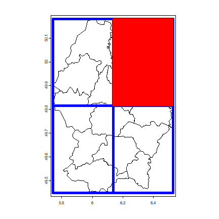
More example data. Object z consists of four polygons; z2 is one
of these four polygons.
z <- rast(p)
dim(z) <- c(2,2)
values(z) <- 1:4
names(z) <- 'Zone'
# coerce SpatRaster to SpatVector polygons
z <- as.polygons(z)
z
## class       : SpatVector
## geometry    : polygons
## dimensions  : 4, 1  (geometries, attributes)
## extent      : 5.74414, 6.528252, 49.44781, 50.18162  (xmin, xmax, ymin, ymax)
## coord. ref. : lon/lat WGS 84 (EPSG:4326)
## names       :  Zone
## type        : <int>
## values      :     1
##                   2
##                   3
##               ...
z2 <- z[2,]
plot(p)
plot(z, add=TRUE, border='blue', lwd=5)
plot(z2, add=TRUE, border='red', lwd=2, col='red')
To append SpatVector objects of the same (vector) type you can use
rbind
b <- rbind(p, z)
head(b)
##   ID_1       NAME_1 ID_2     NAME_2 AREA   POP Zone
## 1    1     Diekirch    1   Clervaux  312 18081   NA
## 2    1     Diekirch    2   Diekirch  218 32543   NA
## 3    1     Diekirch    3    Redange  259 18664   NA
## 4    1     Diekirch    4    Vianden   76  5163   NA
## 5    1     Diekirch    5      Wiltz  263 16735   NA
## 6    2 Grevenmacher    6 Echternach  188 18899   NA
tail(b)
##    ID_1     NAME_1 ID_2     NAME_2 AREA    POP Zone
## 11    3 Luxembourg   10 Luxembourg  237 182607   NA
## 12    3 Luxembourg   11     Mersch  233  32112   NA
## 13  NaN       <NA>  NaN       <NA>  NaN    NaN    1
## 14  NaN       <NA>  NaN       <NA>  NaN    NaN    2
## 15  NaN       <NA>  NaN       <NA>  NaN    NaN    3
## 16  NaN       <NA>  NaN       <NA>  NaN    NaN    4
Note how rbind allows you to append SpatVector objects with
different attribute names, unlike the standard rbind for
data.frames.
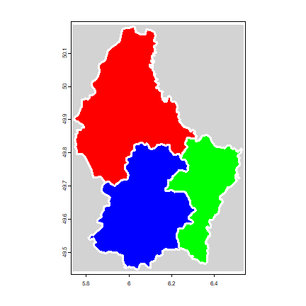
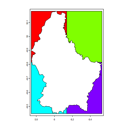
Aggregate
It is common to aggregate (“dissolve”) polygons that have the same value for an attribute of interest. In this case, if we do not care about the second level subdivisions of Luxembourg, we could aggregate by the first level subdivisions.
pa <- aggregate(p, by='NAME_1')
za <- aggregate(z)
plot(za, col='light gray', border='light gray', lwd=5)
plot(pa, add=TRUE, col=rainbow(3), lwd=3, border='white')
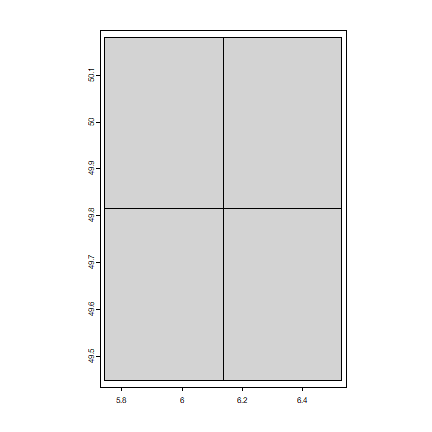
It is also possible to aggregate polygons without dissolving the borders.
zag <- aggregate(z, dissolve=FALSE)
zag
## class       : SpatVector
## geometry    : polygons
## dimensions  : 1, 0  (geometries, attributes)
## extent      : 5.74414, 6.528252, 49.44781, 50.18162  (xmin, xmax, ymin, ymax)
## coord. ref. : lon/lat WGS 84 (EPSG:4326)
plot(zag, col="light gray")
This is a structure that is similar to what you may get for an
archipelago: multiple polygons represented as one entity (one row). Use
disagg to split these up into their parts.
zd <- disagg(zag)
zd
## class       : SpatVector
## geometry    : polygons
## dimensions  : 4, 0  (geometries, attributes)
## extent      : 5.74414, 6.528252, 49.44781, 50.18162  (xmin, xmax, ymin, ymax)
## coord. ref. : lon/lat WGS 84 (EPSG:4326)
Overlay
There are many different ways to “overlay” vector data. Here are some examples:
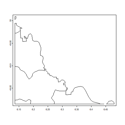
Erase
Erase a part of a SpatVector
e <- erase(p, z2)
plot(e)
Intersect
Intersect SpatVectors
i <- intersect(p, z2)
plot(i)
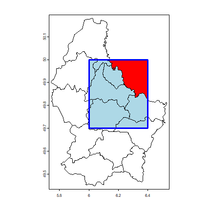
You can also intersect or crop with a SpatExtent (rectangle).
The difference between intersect and crop is that with crop
the geometry of the second argument is not added to the output.
e <- ext(6, 6.4, 49.7, 50)
pe <- crop(p, e)
plot(p)
plot(e, add=TRUE, lwd=3, col="red")
plot(pe, col='light blue', add=TRUE)
plot(e, add=TRUE, lwd=3, border="blue")
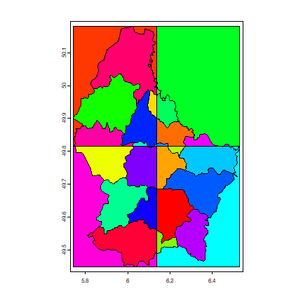
Union
Get the union of two SpatVectors.
u <- union(p, z)
u
## class       : SpatVector
## geometry    : polygons
## dimensions  : 28, 7  (geometries, attributes)
## extent      : 5.74414, 6.528252, 49.44781, 50.18162  (xmin, xmax, ymin, ymax)
## coord. ref. : lon/lat WGS 84 (EPSG:4326)
## names       :  Zone  ID_1 NAME_1  ID_2 NAME_2  AREA   POP
## type        : <int> <num>  <chr> <num>  <chr> <num> <num>
## values      :     1    NA     NA    NA     NA    NA    NA
##                   2    NA     NA    NA     NA    NA    NA
##                   3    NA     NA    NA     NA    NA    NA
##               ...
Note that there are many more polygons now. One for each unique combination of polygons (and attributes in this case).
set.seed(5)
plot(u, col=sample(rainbow(length(u))))
Cover
cover is a combination of intersect and union. intersect
returns new (intersected) geometries with the attributes of both input
datasets. union appends the geometries and attributes of the input.
cover returns the intersection and appends the other geometries and
attributes of both datasets.
cov <- cover(p, z[c(1,4),])
cov
## class       : SpatVector
## geometry    : polygons
## dimensions  : 11, 7  (geometries, attributes)
## extent      : 5.74414, 6.528252, 49.44781, 50.18162  (xmin, xmax, ymin, ymax)
## coord. ref. : lon/lat WGS 84 (EPSG:4326)
## names       :  ID_1   NAME_1  ID_2   NAME_2  AREA   POP  Zone
## type        : <num>    <chr> <num>    <chr> <num> <num> <int>
## values      :     1 Diekirch     1 Clervaux   312 18081    NA
##                   1 Diekirch     2 Diekirch   218 32543    NA
##                   1 Diekirch     3  Redange   259 18664    NA
##               ...
plot(cov)
Difference
The symmetrical difference of two SpatVectors
dif <- symdif(z,p)
plot(dif, col=rainbow(length(dif)))
dif
## class       : SpatVector
## geometry    : polygons
## dimensions  : 4, 1  (geometries, attributes)
## extent      : 5.74414, 6.528252, 49.44781, 50.18162  (xmin, xmax, ymin, ymax)
## coord. ref. : lon/lat WGS 84 (EPSG:4326)
## names       :  Zone
## type        : <int>
## values      :     1
##                   2
##                   3
##               ...
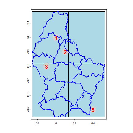
Spatial queries
We can query polygons with points (“point-in-polygon query”).
pts <- matrix(c(6, 6.1, 5.9, 5.7, 6.4, 50, 49.9, 49.8, 49.7, 49.5), ncol=2)
spts <- vect(pts, crs=crs(p))
plot(z, col='light blue', lwd=2)
points(spts, col='light gray', pch=20, cex=6)
text(spts, 1:nrow(pts), col='red', font=2, cex=1.5)
lines(p, col='blue', lwd=2)
extract is used for queries between SpatVector and SpatRaster
objects, and also for queries between SpatVectors.
extract(spts, p)
##       id.y id.x
##  [1,]    1  NaN
##  [2,]    2  NaN
##  [3,]    3  NaN
##  [4,]    4  NaN
##  [5,]    5  NaN
##  [6,]    6  NaN
##  [7,]    7  NaN
##  [8,]    8  NaN
##  [9,]    9  NaN
## [10,]   10  NaN
## [11,]   11  NaN
## [12,]   12  NaN
extract(spts, z)
##      id.y id.x
## [1,]    1  NaN
## [2,]    2  NaN
## [3,]    3  NaN
## [4,]    4  NaN