Coordinate Reference Systems
Introduction
A very important aspect of spatial data is the coordinate reference system (CRS) that is used. For example, a location of (140, 12) is not meaningful if you do know where the origin (0,0) is and if the x-coordinate is 140 meters, feet, nautical miles, kilometers, or perhaps degrees away from the x-origin.
Coordinate Reference Systems (CRS)
Angular coordinates
The earth has an irregular spheroid-like shape. The natural coordinate reference system for geographic data is longitude/latitude. This is an angular coordinate reference system. The latitude \(\phi\) (phi) of a point is the angle between the equatorial plane and the line that passes through a point and the center of the Earth. Longitude \(\lambda\) (lambda) is the angle from a reference meridian (lines of constant longitude) to a meridian that passes through the point.
Obviously we cannot actually measure these angles. But we can estimate them. To do so, you need a model of the shape of the earth. Such a model is called a “datum”. The simplest datums are a spheroid (a sphere that is “flattened” at the poles and bulges at the equator). More complex datums allow for more variation in the earth’s shape. The most commonly used datum is called WGS84 (World Geodesic System 1984). This is very similar to NAD83 (The North American Datum of 1983). Other, local datums exist to more precisely record locations for a single country or region.
So the basic way to record a location is a coordinate pair in degrees and a reference datum. Sometimes people say that their coordinates are “in WGS84”. That does not tell us much; they typically mean to say that they are longitude/latitude relative to the WGS84 datum. Likewise longitude/latitude coordinates are sometimes referred to as “geographic” coordinates. That is rather odd, if planar coordinate reference systems (see below) are not geographic, what are they?
Projections
A major question in spatial analysis and cartography is how to transform this three dimensional angular system to a two dimensional planar (sometimes called “Cartesian”) system. A planar system is easier to use for certain calculations and required to make maps (unless you have a 3-d printer). The different types of planar coordinate reference systems are referred to as “projections”. Examples are “Mercator”, “UTM”, “Robinson”, “Lambert”, “Sinusoidal” and “Albers”.
There is not one best projection. Some projections can be used for a map of the whole world; other projections are appropriate for small areas only. One of the most important characteristics of a map projection is whether it is “equal area” (the scale of the map is constant) or “conformal” (the shapes of the geographic features are as they are seen on a globe). No two dimensional map projection can be both conformal and equal-area (but they can be approximately both for smaller areas, e.g. UTM, or Lambert Equal Area for a larger area), and some are neither.
Notation
A planar CRS is defined by a projection, datum, and a set of parameters. The parameters determine things like where the center of the map is. The number of parameters depends on the projection. It is therefore not trivial to document a projection used, and several systems exist. In R we used to depend on the PROJ.4 notation. PROJ.4 is the name of a software library that is commonly used for CRS transformation.
Here is a list of commonly used projections and their parameters in PROJ4 notation. You can find many more of these on spatialreference.org
The PROJ.4 notation is no longer fully supported in the newer
versions of the library (that was renamed to \(PR\phi J\)). It still
works for CRSs with the WGS84 datum. For other cases you have to use a
EPSG code (if available) or a Well-Known-Text notation.
Most commonly used CRSs have been assigned a “EPSG code” (EPSG stands
for European Petroleum Survey Group). This is a unique ID that can be a
simple way to identify a CRS. For example EPSG:27561 is equivalent
to
+proj=lcc +lat_1=49.5 +lat_0=49.5 +lon_0=0 +k_0=0.999877341 +x_0=6 +y_0=2 +a=6378249.2 +b=6356515
+towgs84=-168,-60,320,0,0,0,0 +pm=paris +units=m +no_defs.
Now let’s look at an example with a spatial data set in R.
library(terra)
## terra 1.9.21
f <- system.file("ex/lux.shp", package="terra")
p <- vect(f)
p
## class       : SpatVector
## geometry    : polygons
## dimensions  : 12, 6  (geometries, attributes)
## extent      : 5.74414, 6.528252, 49.44781, 50.18162  (xmin, xmax, ymin, ymax)
## source      : lux.shp
## coord. ref. : lon/lat WGS 84 (EPSG:4326)
## names       :  ID_1   NAME_1  ID_2   NAME_2  AREA   POP
## type        : <num>    <chr> <num>    <chr> <num> <num>
## values      :     1 Diekirch     1 Clervaux   312 18081
##                   1 Diekirch     2 Diekirch   218 32543
##                   1 Diekirch     3  Redange   259 18664
##               ...
We can inspect the coordinate reference system like this.
crs(p)
## [1] "GEOGCRS[\"WGS 84\",\n    DATUM[\"World Geodetic System 1984\",\n        ELLIPSOID[\"WGS 84\",6378137,298.257223563,\n            LENGTHUNIT[\"metre\",1]]],\n    PRIMEM[\"Greenwich\",0,\n        ANGLEUNIT[\"degree\",0.0174532925199433]],\n    CS[ellipsoidal,2],\n        AXIS[\"geodetic latitude (Lat)\",north,\n            ORDER[1],\n            ANGLEUNIT[\"degree\",0.0174532925199433]],\n        AXIS[\"geodetic longitude (Lon)\",east,\n            ORDER[2],\n            ANGLEUNIT[\"degree\",0.0174532925199433]],\n    ID[\"EPSG\",4326]]"
Assigning a CRS
Sometimes we have data without a CRS. This can be because the file used
was incomplete, or perhaps because we created the data ourselves with R
code. In that case we can assign the CRS if we know what it should
be. Here I first remove the CRS of pp and then I set it again.
pp <- p
crs(pp) <- ""
crs(pp)
## [1] ""
crs(pp) <- "+proj=longlat +datum=WGS84"
crs(pp)
## [1] "GEOGCRS[\"unknown\",\n    DATUM[\"World Geodetic System 1984\",\n        ELLIPSOID[\"WGS 84\",6378137,298.257223563,\n            LENGTHUNIT[\"metre\",1]],\n        ID[\"EPSG\",6326]],\n    PRIMEM[\"Greenwich\",0,\n        ANGLEUNIT[\"degree\",0.0174532925199433],\n        ID[\"EPSG\",8901]],\n    CS[ellipsoidal,2],\n        AXIS[\"longitude\",east,\n            ORDER[1],\n            ANGLEUNIT[\"degree\",0.0174532925199433,\n                ID[\"EPSG\",9122]]],\n        AXIS[\"latitude\",north,\n            ORDER[2],\n            ANGLEUNIT[\"degree\",0.0174532925199433,\n                ID[\"EPSG\",9122]]]]"
Note that you should not use this approach to change the CRS of a data set from what it is to what you want it to be. Assigning a CRS is like labeling something. You need to provide the label that corresponds to the item. Not to what you would like it to be. For example if you label a bicycle, you can write “bicycle”. Perhaps you would prefer a car, and you can label your bicycle as “car” but that would not do you any good. It is still a bicycle. You can try to transform your bicycle into a car. That would not be easy. Transforming spatial data is easier.
Transforming vector data
We can transform these data to a new data set with another CRS using the
project method.
Here we use the Robinson projection. First we need to find the correct notation.
newcrs <- "+proj=robin +datum=WGS84"
Now use it
rob <- terra::project(p, newcrs)
rob
## class       : SpatVector
## geometry    : polygons
## dimensions  : 12, 6  (geometries, attributes)
## extent      : 471320.7, 536010.5, 5269709, 5345677  (xmin, xmax, ymin, ymax)
## coord. ref. : +proj=robin +lon_0=0 +x_0=0 +y_0=0 +datum=WGS84 +units=m +no_defs
## names       :  ID_1   NAME_1  ID_2   NAME_2  AREA   POP
## type        : <num>    <chr> <num>    <chr> <num> <num>
## values      :     1 Diekirch     1 Clervaux   312 18081
##                   1 Diekirch     2 Diekirch   218 32543
##                   1 Diekirch     3  Redange   259 18664
##               ...
After the transformation, the units of the geometry are no longer in degrees, but in meters away from (longitude=0, latitude=0). The spatial extent of the data is also in these units.
We can backtransform to longitude/latitude:
p2 <- terra::project(rob, "+proj=longlat +datum=WGS84")
Transforming raster data
Vector data can be transformed from lon/lat coordinates to planar and back without loss of precision. This is not the case with raster data. A raster consists of rectangular cells of the same size (in terms of the units of the CRS; their actual size may vary). It is not possible to transform cell by cell. For each new cell, values need to be estimated based on the values in the overlapping old cells. If the values are categorical data, the “nearest neighbor” method is commonly used. Otherwise some sort of interpolation is employed (e.g. “bilinear”).
Because projection of rasters affects the cell values, in most cases you will want to avoid projecting raster data and rather project vector data. But here is how you can project raster data.
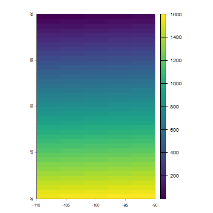
r <- rast(xmin=-110, xmax=-90, ymin=40, ymax=60, ncols=40, nrows=40)
values(r) <- 1:ncell(r)
r
## class       : SpatRaster
## size        : 40, 40, 1  (nrow, ncol, nlyr)
## resolution  : 0.5, 0.5  (x, y)
## extent      : -110, -90, 40, 60  (xmin, xmax, ymin, ymax)
## coord. ref. : lon/lat WGS 84 (CRS84) (OGC:CRS84)
## source(s)   : memory
## name        : lyr.1
## min value   :     1
## max value   :  1600
plot(r)
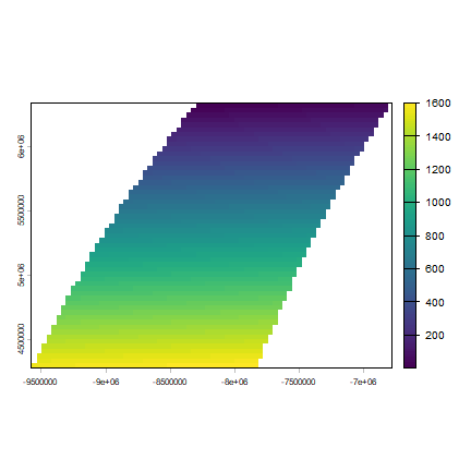
The simplest approach is to provide a new crs (the Robinson crs in this case)
newcrs
## [1] "+proj=robin +datum=WGS84"
pr1 <- terra::project(r, newcrs)
crs(pr1)
## [1] "PROJCRS[\"unknown\",\n    BASEGEOGCRS[\"unknown\",\n        DATUM[\"World Geodetic System 1984\",\n            ELLIPSOID[\"WGS 84\",6378137,298.257223563,\n                LENGTHUNIT[\"metre\",1]],\n            ID[\"EPSG\",6326]],\n        PRIMEM[\"Greenwich\",0,\n            ANGLEUNIT[\"degree\",0.0174532925199433],\n            ID[\"EPSG\",8901]]],\n    CONVERSION[\"unknown\",\n        METHOD[\"Robinson\"],\n        PARAMETER[\"Longitude of natural origin\",0,\n            ANGLEUNIT[\"degree\",0.0174532925199433],\n            ID[\"EPSG\",8802]],\n        PARAMETER[\"False easting\",0,\n            LENGTHUNIT[\"metre\",1],\n            ID[\"EPSG\",8806]],\n        PARAMETER[\"False northing\",0,\n            LENGTHUNIT[\"metre\",1],\n            ID[\"EPSG\",8807]]],\n    CS[Cartesian,2],\n        AXIS[\"(E)\",east,\n            ORDER[1],\n            LENGTHUNIT[\"metre\",1,\n                ID[\"EPSG\",9001]]],\n        AXIS[\"(N)\",north,\n            ORDER[2],\n            LENGTHUNIT[\"metre\",1,\n                ID[\"EPSG\",9001]]]]"
plot(pr1)
But that is not a good method. As you should want to assure that you project to exactly the raster parameters you need (so that it lines up with other raster data you are using).
To have this kind of control, provide an existing SpatRaster with the geometry you desire. That is generally the best way to project raster. By providing an existing SpatRaster, such that your newly projected data perfectly aligns with it. In this example we do not have an existing SpatRaster object, so we create from the result obtained above.
x <- rast(pr1)
# Set the cell size
res(x) <- 200000
Now project, and note the change in the coordinates.
pr3 <- terra::project(r, x)
pr3
## class       : SpatRaster
## size        : 10, 14, 1  (nrow, ncol, nlyr)
## resolution  : 200000, 200000  (x, y)
## extent      : -9577685, -6777685, 4283463, 6283463  (xmin, xmax, ymin, ymax)
## coord. ref. : +proj=robin +lon_0=0 +x_0=0 +y_0=0 +datum=WGS84 +units=m +no_defs
## source(s)   : memory
## name        :      lyr.1
## min value   : 111.154106
## max value   : 1523.57959
plot(pr3)
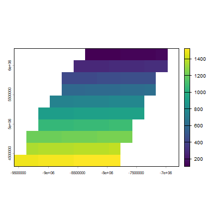
For raster based analysis it is often important to use equal area projections, particularly when large areas are analyzed. This will assure that the grid cells are all of same size, and therefore comparable to each other, especially when count data are used.