Vector data
Introduction
The terra package defines a set of classes to represent spatial
data. A class defines a particular data type. The data.frame is an
example of a class. Any particular data.frame you create is an
object (instantiation) of that class.
The main reason for defining classes is to create a standard representation of a particular data type to make it easier to write functions (known as “methods”) for them. See Hadley Wickham’s Advanced R or John Chambers’ Software for data analysis for a detailed discussion of the use of classes in R.
terra introduces a number of classes with names that start with
Spat. For vector data, the relevant class is SpatVector. These
classes represent geometries as well as attributes (variables)
describing the geometries.
It is possible to create SpatVector objects from scratch with R
code. This is very useful when creating a small self contained example
to illustrate something, for example to ask a question about how to do a
particular operation; without needing to give access to the real data
you are using (which is always cumbersome). It is also frequently done
when using coordinates that were obtained with a GPS. But in most other
cases, you will read these from a file or database, see Chapter
5 for examples.
To get started, let’s make some SpatVector objects from scratch anyway, using the same data as were used in the previous chapter.
Points
longitude <- c(-116.7, -120.4, -116.7, -113.5, -115.5, -120.8, -119.5, -113.7, -113.7, -110.7)
latitude <- c(45.3, 42.6, 38.9, 42.1, 35.7, 38.9, 36.2, 39, 41.6, 36.9)
lonlat <- cbind(longitude, latitude)
Now create a SpatVector object. First load the terra package
from the library. If this command fails with
Error in library(terra) : there is no package called ‘terra’, then
you need to install the package first, with
install.packages("terra")
library(terra)
## terra 1.9.21
##
## Attaching package: 'terra'
## The following object is masked from 'package:knitr':
##
##     spin
pts <- vect(lonlat)
Let’s check what kind of object pts is.
class (pts)
## [1] "SpatVector"
## attr(,"package")
## [1] "terra"
And what is inside of it
pts
## class       : SpatVector
## geometry    : points
## dimensions  : 10, 0  (geometries, attributes)
## extent      : -120.8, -110.7, 35.7, 45.3  (xmin, xmax, ymin, ymax)
## coord. ref. :
geom(pts)
##       geom part      x    y hole
##  [1,]    1    1 -116.7 45.3    0
##  [2,]    2    1 -120.4 42.6    0
##  [3,]    3    1 -116.7 38.9    0
##  [4,]    4    1 -113.5 42.1    0
##  [5,]    5    1 -115.5 35.7    0
##  [6,]    6    1 -120.8 38.9    0
##  [7,]    7    1 -119.5 36.2    0
##  [8,]    8    1 -113.7 39.0    0
##  [9,]    9    1 -113.7 41.6    0
## [10,]   10    1 -110.7 36.9    0
So we see that the object has the coordinates we supplied, but also an
extent. This spatial extent was computed from the coordinates. There
is also a coordinate reference system (“CRS”, discussed in more detail
later). We did not provide the CRS when we created pts. That is not
good, so let’s recreate the object, and now provide a CRS.
crdref <- "+proj=longlat +datum=WGS84"
pts <- vect(lonlat, crs=crdref)
pts
## class       : SpatVector
## geometry    : points
## dimensions  : 10, 0  (geometries, attributes)
## extent      : -120.8, -110.7, 35.7, 45.3  (xmin, xmax, ymin, ymax)
## coord. ref. : +proj=longlat +datum=WGS84 +no_defs
crs(pts)
## [1] "GEOGCRS[\"unknown\",\n    DATUM[\"World Geodetic System 1984\",\n        ELLIPSOID[\"WGS 84\",6378137,298.257223563,\n            LENGTHUNIT[\"metre\",1]],\n        ID[\"EPSG\",6326]],\n    PRIMEM[\"Greenwich\",0,\n        ANGLEUNIT[\"degree\",0.0174532925199433],\n        ID[\"EPSG\",8901]],\n    CS[ellipsoidal,2],\n        AXIS[\"longitude\",east,\n            ORDER[1],\n            ANGLEUNIT[\"degree\",0.0174532925199433,\n                ID[\"EPSG\",9122]]],\n        AXIS[\"latitude\",north,\n            ORDER[2],\n            ANGLEUNIT[\"degree\",0.0174532925199433,\n                ID[\"EPSG\",9122]]]]"
We can add attributes (variables) to the SpatVector object. First we
need a data.frame with the same number of rows as there are
geometries.
# Generate random precipitation values, same quantity as points
precipvalue <- runif(nrow(lonlat), min=0, max=100)
df <- data.frame(ID=1:nrow(lonlat), precip=precipvalue)
Combine the SpatVector with the data.frame.
ptv <- vect(lonlat, atts=df, crs=crdref)
To see what is inside:
ptv
## class       : SpatVector
## geometry    : points
## dimensions  : 10, 2  (geometries, attributes)
## extent      : -120.8, -110.7, 35.7, 45.3  (xmin, xmax, ymin, ymax)
## coord. ref. : +proj=longlat +datum=WGS84 +no_defs
## names       :    ID  precip
## type        : <int>   <num>
## values      :     1 40.6682
##                   2 3.49299
##                   3 37.3135
##               ...
Lines and polygons
Making a SpatVector of points was easy. Making a SpatVector of
lines or polygons is a bit more complex, but stil relatively
straightforward.
lon <- c(-116.8, -114.2, -112.9, -111.9, -114.2, -115.4, -117.7)
lat <- c(41.3, 42.9, 42.4, 39.8, 37.6, 38.3, 37.6)
lonlat <- cbind(id=1, part=1, lon, lat)
lonlat
##      id part    lon  lat
## [1,]  1    1 -116.8 41.3
## [2,]  1    1 -114.2 42.9
## [3,]  1    1 -112.9 42.4
## [4,]  1    1 -111.9 39.8
## [5,]  1    1 -114.2 37.6
## [6,]  1    1 -115.4 38.3
## [7,]  1    1 -117.7 37.6
lns <- vect(lonlat, type="lines", crs=crdref)
lns
## class       : SpatVector
## geometry    : lines
## dimensions  : 1, 0  (geometries, attributes)
## extent      : -117.7, -111.9, 37.6, 42.9  (xmin, xmax, ymin, ymax)
## coord. ref. : +proj=longlat +datum=WGS84 +no_defs
pols <- vect(lonlat, type="polygons", crs=crdref)
pols
## class       : SpatVector
## geometry    : polygons
## dimensions  : 1, 0  (geometries, attributes)
## extent      : -117.7, -111.9, 37.6, 42.9  (xmin, xmax, ymin, ymax)
## coord. ref. : +proj=longlat +datum=WGS84 +no_defs
Behind the scenes the class deals with the complexity of accommodating
for the possibility of multiple polygons, each consisting of multiple
sub-polygons, some of which may be “holes”. You do not need to
understand how these structures are organized. The main take home
message is that a SpatVector stores geometries (coordinates), the
name of the coordinate reference system, and attributes.
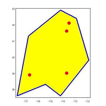
We can make use plot to make a map.
plot(pols, las=1)
plot(pols, border='blue', col='yellow', lwd=3, add=TRUE)
points(pts, col='red', pch=20, cex=3)
We’ll make more fancy maps later.