Data preparation
Species occurrence data
Importing occurrence data into R is easy. But collecting, georeferencing, and cross-checking coordinate data is tedious. Discussions about species distribution modeling often focus on comparing modeling methods, but if you are dealing with species with few and uncertain records, your focus probably ought to be on improving the quality of the occurrence data (Lobo, 2008). All methods do better if your occurrence data is unbiased and free of error (Graham et al., 2007) and you have a relatively large number of records (Wisz et al., 2008). While we’ll show you some useful data preparation steps you can do in R, it is necessary to use additional tools as well. For example, QGIS, is a very useful program for interactive editing of point data sets.
Importing occurrence data
In most cases you will have a file with point locality data representing
the known distribution of a species. Below is an example of using
read.table to read records that are stored in a text file.
We are using an example file that is installed with the dismo
package, and for that reason we use a complex way to construct the
filename, but you can replace that with your own filename. (remember to
use forward slashes in the path of filenames!). system.file inserts
the file path to where dismo is installed. If you haven’t used the
paste function before, it’s worth familiarizing yourself with it
(type ?pastein the command window).
# loads the dismo library
library(dismo)
file <- paste0(system.file(package="dismo"), "/ex/bradypus.csv")
# this is the file we will use:
file
## [1] "C:/soft/R/R-devel/library/dismo/ex/bradypus.csv"
Now read it and inspect the values of the file
bradypus <- read.table(file,  header=TRUE,  sep=",")
# or do:  bradypus <- read.csv(file)
# first rows
head(bradypus)
##               species      lon      lat
## 1 Bradypus variegatus -65.4000 -10.3833
## 2 Bradypus variegatus -65.3833 -10.3833
## 3 Bradypus variegatus -65.1333 -16.8000
## 4 Bradypus variegatus -63.6667 -17.4500
## 5 Bradypus variegatus -63.8500 -17.4000
## 6 Bradypus variegatus -64.4167 -16.0000
# we only need columns 2 and 3:
bradypus <- bradypus[,2:3]
head(bradypus)
##        lon      lat
## 1 -65.4000 -10.3833
## 2 -65.3833 -10.3833
## 3 -65.1333 -16.8000
## 4 -63.6667 -17.4500
## 5 -63.8500 -17.4000
## 6 -64.4167 -16.0000
You can also read such data directly out of Excel files or from a
database (see e.g. the RODBC package). Because this is a csv (comma
separated values) file, we could also have used the read.csv
function. No matter how you do it, the objective is to get a matrix (or
a data.frame) with at least 2 columns that hold the coordinates of
the locations where a species was observed. Coordinates are typically
expressed as longitude and latitude (i.e. angular), but they could also
be Easting and Northing in UTM or another planar coordinate reference
system (map projection). The convention used here is to organize the
coordinates columns so that longitude is the first and latitude the
second column (think x and y axes in a plot; longitude is x, latitude is
y); they often are in the reverse order, leading to undesired results.
In many cases you will have additional columns, e.g., a column to
indicate the species if you are modeling multiple species; and a column
to indicate whether this is a ‘presence’ or an ‘absence’ record (a much
used convention is to code presence with a 1 and absence with a 0).
If you do not have any species distribution data you can get started by
downloading data from the Global Biodiversity Inventory Facility
(GBIF). In the dismo package there is a
function gbif that you can use for this. The data used below were
downloaded (and saved to a permanent data set for use in this vignette)
using the gbif function like this:
acaule <- gbif("solanum", "acaule*", geo=FALSE)
If you want to understand the order of the arguments given here to
gbif or find out what other arguments you can use with this
function, check out the help file (remember you can’t access help files
if the library is not loaded), by typing: ?gbif or help(gbif).
Note the use of the asterix in “acaule*” to not only request
Solanum acaule, but also variations such as the full name,*Solanum
acaule* Bitter, or subspecies such as Solanum acaule subsp.
aemulans.
Many occurence records may not have geographic coordinates. In this case, out of the 1366 records that GBIF returned (January 2013), there were 1082 records with coordinates (this was 699 and 54 in March 2010, a tremendous improvement!)
# load the saved S. acaule data
data(acaule)
# how many rows and colums?
dim(acaule)
## [1] 1366   25
#select the records that have longitude and latitude data
colnames(acaule)
##  [1] "species"               "continent"             "country"
##  [4] "adm1"                  "adm2"                  "locality"
##  [7] "lat"                   "lon"                   "coordUncertaintyM"
## [10] "alt"                   "institution"           "collection"
## [13] "catalogNumber"         "basisOfRecord"         "collector"
## [16] "earliestDateCollected" "latestDateCollected"   "gbifNotes"
## [19] "downloadDate"          "maxElevationM"         "minElevationM"
## [22] "maxDepthM"             "minDepthM"             "ISO2"
## [25] "cloc"
acgeo <- subset(acaule, !is.na(lon) & !is.na(lat))
dim(acgeo)
## [1] 1082   25
# show some values
acgeo[1:4, c(1:5,7:10)]
##                    species     continent   country  adm1           adm2
## 1    Solanum acaule Bitter South America Argentina Jujuy Santa Catalina
## 2    Solanum acaule Bitter South America      Peru Cusco        Canchis
## 3 Solanum acaule f. acaule          <NA> Argentina  <NA>           <NA>
## 4 Solanum acaule f. acaule          <NA>   Bolivia  <NA>           <NA>
##        lat      lon coordUncertaintyM  alt
## 1 -21.9000 -66.1000              <NA>  NaN
## 2 -13.5000 -71.0000              <NA> 4500
## 3 -22.2666 -65.1333              <NA> 3800
## 4 -18.6333 -66.9500              <NA> 3700
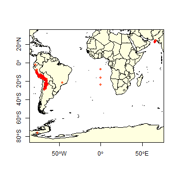
Below is a simple way to make a map of the occurrence localities of Solanum acaule. It is important to make such maps to assure that the points are, at least roughly, in the right location.
library(maptools)
data(wrld_simpl)
plot(wrld_simpl, xlim=c(-80,70), ylim=c(-60,10), axes=TRUE, col="light yellow")
# restore the box around the map
box()
# add the points
points(acgeo$lon, acgeo$lat, col='orange', pch=20, cex=0.75)
# plot points again to add a border, for better visibility
points(acgeo$lon, acgeo$lat, col='red', cex=0.75)
The wrld_simpl dataset contains rough country outlines. You can use
other datasets of polygons (or lines or points) as well. For example,
you can download higher resolution data country and subnational
administrative boundaries data with the getData function of the
raster package. You can also read your own shapefile data into R
using the shapefile function in the raster package.
Data cleaning
Data ‘cleaning’ is particularly important for data sourced from species distribution data warehouses such as GBIF. Such efforts do not specifically gather data for the purpose of species distribution modeling, so you need to understand the data and clean them appropriately, for your application. Here we provide an example.
Solanum acaule is a species that occurs in the higher parts of the
Andes mountains of southern Peru, Bolivia and northern Argentina. Do you
see any errors on the map?
There are a few records that map in the ocean just south of Pakistan. Any idea why that may have happened? It is a common mistake, missing minus signs. The coordinates are around (65.4, 23.4) but they should in Northern Argentina, around (-65.4, -23.4) (you can use the “click” function to query the coordintates on the map). There are two records (rows 303 and 885) that map to the same spot in Antarctica (-76.3, -76.3). The locality description says that is should be in Huarochiri, near Lima, Peru. So the longitude is probably correct, and erroneously copied to the latitude. Interestingly the record occurs twice. The orignal source is the International Potato Center, and a copy is provided by “SINGER” that aling the way appears to have “corrected” the country to Antarctica:
acaule[c(303,885),1:10]
##                          species continent    country adm1 adm2
## 303        solanum acaule acaule      <NA> Antarctica <NA> <NA>
## 885 solanum acaule acaule BITTER      <NA>       Peru <NA> <NA>
##                         locality   lat   lon coordUncertaintyM  alt
## 303                         <NA> -76.3 -76.3              <NA>  NaN
## 885 Lima P. Huarochiri Pacomanta -76.3 -76.3              <NA> 3800
The point in Brazil (record acaule[98,]) should be in soutern Bolivia,
so this is probably due to a typo in the longitude. Likewise, there are
also three records that have plausible latitudes, but longitudes that
are clearly wrong, as they are in the Atlantic Ocean, south of West
Africa. It looks like they have a longitude that is zero. In many
data-bases you will find values that are ‘zero’ where ‘no data’ was
intended. The gbif function (when using the default arguments) sets
coordinates that are (0, 0) to NA, but not if one of the coordinates
is zero. Let’s see if we find them by searching for records with
longitudes of zero.
Let’s have a look at these records:
lonzero = subset(acgeo, lon==0)
# show all records, only the first 13 columns
lonzero[, 1:13]
##                                  species continent   country adm1 adm2
## 1159 Solanum acaule Bitter subsp. acaule      <NA> Argentina <NA> <NA>
## 1160 Solanum acaule Bitter subsp. acaule      <NA>   Bolivia <NA> <NA>
## 1161 Solanum acaule Bitter subsp. acaule      <NA>      Peru <NA> <NA>
## 1162 Solanum acaule Bitter subsp. acaule      <NA>      Peru <NA> <NA>
## 1163 Solanum acaule Bitter subsp. acaule      <NA> Argentina <NA> <NA>
## 1164 Solanum acaule Bitter subsp. acaule      <NA>   Bolivia <NA> <NA>
##                                              locality        lat lon
## 1159 between Quelbrada del Chorro and Laguna Colorada -23.716667   0
## 1160                                            Llave -16.083334   0
## 1161                    km 205 between Puno and Cuzco  -6.983333   0
## 1162                    km 205 between Puno and Cuzco  -6.983333   0
## 1163 between Quelbrada del Chorro and Laguna Colorada -23.716667   0
## 1164                                            Llave -16.083334   0
##      coordUncertaintyM  alt institution collection catalogNumber
## 1159              <NA> 3400         IPK         GB     WKS 30027
## 1160              <NA> 3900         IPK         GB     WKS 30050
## 1161              <NA> 4250         IPK  WKS 30048        304709
## 1162              <NA> 4250         IPK         GB     WKS 30048
## 1163              <NA> 3400         IPK  WKS 30027        304688
## 1164              <NA> 3900         IPK  WKS 30050        304711
The records are from Bolivia, Peru and Argentina, confirming that
coordinates are in error. Alternatively, it could have been that the
coordinates were correct, perhaps referring to a location in the
Atlantic Ocean where a fish was caught rather than a place where S.
acaule was collected). Records with the wrong species name can be among
the hardest to correct (e.g., distinguishing between brown bears and
sasquatch, Lozier et al., 2009). The one record in Ecuador is like
that, there is some debate whether that is actually a specimen of
S. albicans or an anomalous hexaploid variety of S. acaule.
Duplicate records
Interestingly, another data quality issue is revealed above: each record in ‘lonzero’ occurs twice. This could happen because plant samples are often split and send to multiple herbariums. But in this case it seems that the IPK (The Leibniz Institute of Plant Genetics and Crop Plant Research) provided these data twice to the GBIF database (perhaps from seperate databases at IPK?). The function ‘duplicated’ can sometimes be used to remove duplicates.
# which records are duplicates (only for the first 10 columns)?
dups <- duplicated(lonzero[, 1:10])
# remove duplicates
lonzero  <-  lonzero[dups, ]
lonzero[,1:13]
##                                  species continent   country adm1 adm2
## 1162 Solanum acaule Bitter subsp. acaule      <NA>      Peru <NA> <NA>
## 1163 Solanum acaule Bitter subsp. acaule      <NA> Argentina <NA> <NA>
## 1164 Solanum acaule Bitter subsp. acaule      <NA>   Bolivia <NA> <NA>
##                                              locality        lat lon
## 1162                    km 205 between Puno and Cuzco  -6.983333   0
## 1163 between Quelbrada del Chorro and Laguna Colorada -23.716667   0
## 1164                                            Llave -16.083334   0
##      coordUncertaintyM  alt institution collection catalogNumber
## 1162              <NA> 4250         IPK         GB     WKS 30048
## 1163              <NA> 3400         IPK  WKS 30027        304688
## 1164              <NA> 3900         IPK  WKS 30050        304711
Another approach might be to detect duplicates for the same species and some coordinates in the data, even if the records were from collections by different people or in different years. (in our case, using species is redundant as we have data for only one species)
# differentiating by (sub) species
# dups2 <- duplicated(acgeo[, c('species', 'lon', 'lat')])
# ignoring (sub) species and other naming variation
dups2 <- duplicated(acgeo[, c('lon', 'lat')])
# number of duplicates
sum(dups2)
## [1] 483
# keep the records that are _not_ duplicated
acg <- acgeo[!dups2, ]
Let’s repatriate the records near Pakistan to Argentina, and remove the records in Brazil, Antarctica, and with longitude=0
i <- acg$lon > 0 & acg$lat > 0
acg$lon[i] <- -1 * acg$lon[i]
acg$lat[i] <- -1 * acg$lat[i]
acg <- acg[acg$lon < -50 & acg$lat > -50, ]
Cross-checking
It is important to cross-check coordinates by visual and other means.
One approach is to compare the country (and lower level administrative
subdivisions) of the site as specified by the records, with the country
implied by the coordinates (Hijmans et al., 1999). In the example
below we use the coordinates function from the sp package to
create a SpatialPointsDataFrame, and then the over function,
also from sp, to do a point-in-polygon query with the countries
polygons.
We can make a SpatialPointsDataFrame using the statistical function notation (with a tilde):
library(sp)
coordinates(acg) <- ~lon+lat
crs(acg) <- crs(wrld_simpl)
class(acg)
## [1] "SpatialPointsDataFrame"
## attr(,"package")
## [1] "sp"
We can now use the coordinates to do a spatial query of the polygons in wrld_simpl (a SpatialPolygonsDataFrame)
class(wrld_simpl)
## [1] "SpatialPolygonsDataFrame"
## attr(,"package")
## [1] "sp"
ovr <- over(acg, wrld_simpl)
Object ‘ov’ has, for each point, the matching record from wrld_simpl. We need the variable ‘NAME’ in the data.frame of wrld_simpl
head(ovr)
##   FIPS ISO2 ISO3  UN      NAME   AREA  POP2005 REGION SUBREGION     LON     LAT
## 1   AR   AR  ARG  32 Argentina 273669 38747148     19         5 -65.167 -35.377
## 2   PE   PE  PER 604      Peru 128000 27274266     19         5 -75.552  -9.326
## 3   AR   AR  ARG  32 Argentina 273669 38747148     19         5 -65.167 -35.377
## 4   BL   BO  BOL  68   Bolivia 108438  9182015     19         5 -64.671 -16.715
## 5   BL   BO  BOL  68   Bolivia 108438  9182015     19         5 -64.671 -16.715
## 6   BL   BO  BOL  68   Bolivia 108438  9182015     19         5 -64.671 -16.715
cntr <- ovr$NAME
We should ask these two questions: (1) Which points (identified by their record numbers) do not match any country (that is, they are in an ocean)? (There are none (because we already removed the points that mapped in the ocean)). (2) Which points have coordinates that are in a different country than listed in the ‘country’ field of the gbif record
i <- which(is.na(cntr))
i
## integer(0)
j <- which(cntr != acg$country)
# for the mismatches, bind the country names of the polygons and points
cbind(cntr, acg$country)[j,]
##      cntr
## [1,] "27"  "Argentina"
## [2,] "172" "Bolivia"
## [3,] "172" "Bolivia"
## [4,] "172" "Bolivia"
In this case the mismatch is probably because wrld_simpl is not very precise as the records map to locations very close to the border between Bolivia and its neighbors.
plot(acg)
plot(wrld_simpl, add=T, border='blue', lwd=2)
points(acg[j, ], col='red', pch=20, cex=2)
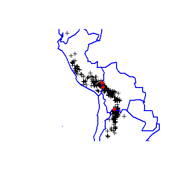
See the sp package for more information on the over function. The
wrld_simpl polygons that we used in the example above are not very
precise, and they probably should not be used in a real analysis. See
GADM for more detailed administrative
division files, or use the getData function from the raster package
(e.g. getData('gadm', country='BOL', level=0) to get the national
borders of Bolivia; and getData('countries') to get all country
boundaries).
Georeferencing
If you have records with locality descriptions but no coordinates, you should consider georeferencing these. Not all the records can be georeferenced. Sometimes even the country is unknown (country==“UNK”). Here we select only records that do not have coordinates, but that do have a locality description.
georef <- subset(acaule, (is.na(lon) | is.na(lat)) & ! is.na(locality) )
dim(georef)
## [1] 131  25
georef[1:3,1:13]
##                          species continent country adm1 adm2
## 606 solanum acaule acaule BITTER      <NA> Bolivia <NA> <NA>
## 607 solanum acaule acaule BITTER      <NA>    Peru <NA> <NA>
## 618 solanum acaule acaule BITTER      <NA>    Peru <NA> <NA>
##                                                                  locality lat
## 606 La Paz P. Franz Tamayo Viscachani 3 km from Huaylapuquio to Pelechuco  NA
## 607                                    Puno P. San Roman Near Tinco Palca  NA
## 618                                              Puno P. Lampa Saraccocha  NA
##     lon coordUncertaintyM  alt institution              collection
## 606  NA              <NA> 4000      PER001 CIP - Potato collection
## 607  NA              <NA> 4000      PER001 CIP - Potato collection
## 618  NA              <NA> 4100      PER001 CIP - Potato collection
##     catalogNumber
## 606    CIP-762165
## 607    CIP-761962
## 618    CIP-762376
For georeferencing, you can try to use the dismo package function
geocode that sends requests to the Google API (this used to be
simple, but these days you need to first get an “API_KEY” from Google).
We demonstrate below, but its use is generally not recommended because
for accurate georeferencing you need a detailed map interface, and
ideally one that allows you to capture the uncertainty associated with
each georeference (Wieczorek et al., 2004).
Here is an example for one of the records with longitude = 0, using Google’s geocoding service. We put the function into a ‘try’ function, to assure elegant error handling if the computer is not connected to the Internet. Note that we use the “cloc” (concatenated locality) field.
georef$cloc[4]
## [1] "Ayacucho P. Huamanga Minas Ckucho, Peru"
#b <- geocode(georef$cloc[4], geo_key="abcdef" )
#b
Before using the geocode function it is best to write the records to a table and “clean” them in a spreadsheet. Cleaning involves translation, expanding abbreviations, correcting misspellings, and making duplicates exactly the same so that they can be georeferenced only once. Then read the the table back into R, and create unique localities, georeference these and merge them with the original data.
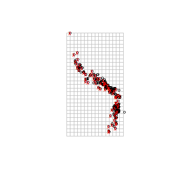
Sampling bias
Sampling bias is frequently present in occurrence records (Hijmans et al., 2001). One can attempt to remove some of the bias by subsampling records, and this is illustrated below. However, subsampling reduces the number of records, and it cannot correct the data for areas that have not been sampled at all. It also suffers from the problem that locally dense records might in fact be a true reflection of the relative suitable of habitat. As in many steps in SDM, you need to understand something about your data and species to implement them well. See Phillips et al. (2009) for an approach with MaxEnt to deal with bias in occurrence records for a group of species.
# create a RasterLayer with the extent of acgeo
r <- raster(acg)
# set the resolution of the cells to (for example) 1 degree
res(r) <- 1
# expand (extend) the extent of the RasterLayer a little
r <- extend(r, extent(r)+1)
# sample:
acsel <- gridSample(acg, r, n=1)
# to illustrate the method and show the result
p <- rasterToPolygons(r)
plot(p, border='gray')
points(acg)
# selected points in red
points(acsel, cex=1, col='red', pch='x')
Note that with the gridSample function you can also do ‘chess-board’
sampling. This can be useful to split the data in ‘training’ and
‘testing’ sets (see the model evaluation chapter).
At this point, it could be useful to save the cleaned data set. For
example with the function write.table or write.csv so that we
can use them later. We did that, and the saved file is available through
dismo and can be retrieved like this:
file <- paste(system.file(package="dismo"), '/ex/acaule.csv', sep='')
acsel <- read.csv(file)
In a real research project you would want to spend much more time on this first data-cleaning and completion step, partly with R, but also with other programs.
##2.8 Exercises
Use the gbif function to download records for the African elephant (or another species of your preference, try to get one with between 10 and 100 records). Use option “geo=FALSE” to also get records with no (numerical) georeference.
Summarize the data: how many records are there, how many have coordinates, how many records without coordinates have a textual georeference (locality description)?
Use the ‘geocode’ function to georeference up to 10 records without coordinates
Make a simple map of all the records, using a color and symbol to distinguish between the coordinates from gbif and the ones returned by Google (via the geocode function). Use ‘gmap’ to create a basemap.
Do you think the observations are a reasonable representation of the distribution (and ecological niche) of the species?
More advanced:
Use the ‘rasterize’ function to create a raster of the number of observations and make a map. Use “wrld_simpl” from the maptools package for country boundaries.
Map the uncertainty associated with the georeferences. Some records in data returned by gbif have that. You can also extract it from the data returned by the geocode function.