Environmental data
Raster data
In species distribution modeling, predictor variables are typically
organized as raster (grid) type files. The predictors should be layers
in a SpatRaster representing variables of interest such as climate,
soil, terrain, vegetation, or land use. These data are typically stored
in files in some kind of geospatial format. Almost all relevant formats
can be used (including geoTiff, netCDF, and Arc-ASCII). Avoid ASCII
files if you can, as they tend to considerably slow down processing
speed. For any particular study the layers should all have the same
spatial extent, resolution, origin, and projection. If necessary, use
functions like crop, extend, aggregate, resample, and
project from the terra package. See the Introduction to spatial
data manipulation for more
information about function you can use to prepare your predictor
variable data. See the help files of the terra package for more info on
how to do this.
The set of predictor variables (rasters) can be used to make a
SpatRaster, which has many layers (see the Spatial Data
tutorial for more info.
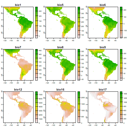
Here we make a list of files that are installed with the predicts package and then create a SpatRaster from these, show the names of each layer, and finally plot them all.
First get the folder with our files. Here we use a file that ships with R.
library(predicts)
## Loading required package: terra
## terra 1.9.21
f <- system.file("ex/bio.tif", package="predicts")
predictors <- rast(f)
predictors
## class       : SpatRaster
## size        : 192, 186, 9  (nrow, ncol, nlyr)
## resolution  : 0.5, 0.5  (x, y)
## extent      : -125, -32, -56, 40  (xmin, xmax, ymin, ymax)
## coord. ref. : lon/lat WGS 84 (EPSG:4326)
## source      : bio.tif
## names       : bio1, bio5, bio6, bio7, bio8, bio9, ...
## min values  :  -23,   61, -212,   60,  -66,  -23, ...
## max values  :  289,  422,  242,  461,  323,  289, ...
names(predictors)
## [1] "bio1"  "bio5"  "bio6"  "bio7"  "bio8"  "bio9"  "bio12" "bio16" "bio17"
plot(predictors)
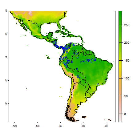
We can also make a plot of a single layer in a SpatRaster, and plot some additional data on top of it. First get the world boundaries and the Bradypus data:
library(geodata)
wrld <- world(path=".")
file <- paste(system.file(package="predicts"), "/ex/bradypus.csv", sep="")
bradypus <- read.table(file,  header=TRUE,  sep=',')
# we do not need the first column
bradypus  <- bradypus[,-1]
And now plot:
# first layer of the SpatRaster
plot(predictors, 1)
lines(wrld)
points(bradypus, col='blue')
The example above uses data representing ‘bioclimatic variables’ from
the WorldClim database (Hijmans et al.,
2004). You can download more recent versions of WorldClim with the
geodata package.
Predictor variable selection can be important, particularly if the
objective of a study is explanation. See, e.g., Austin and Smith (1987),
Austin (2002), Mellert et al., (2011). The early applications of
species modeling tended to focus on explanation (Elith and Leathwick
2009). Nowadays, the objective of SDM tends to be prediction. For
prediction within the same geographic area, variable selection might
arguably be relatively less important, but for many prediction tasks
(e.g. to new times or places, see below) variable selection is
critically important. In all cases it is important to use variables that
are relevant to the ecology of the species (rather than with the first
dataset that can be found on the web!). In some cases it can be useful
to develop new, more ecologically relevant, predictor variables from
existing data. For example, one could use land cover data and the
focal function in the raster package to create a new variable
that indicates how much forest area is available within x km of a grid
cell, for a species that might have a home range of x.
Extracting values from rasters
We now have a set of predictor variables (rasters) and occurrence
points. The next step is to extract the values of the predictors at the
locations of the points. (This step can be skipped for the modeling
methods that are implemented in the dismo package). This is a very
straightforward thing to do using the ‘extract’ function from the raster
package. In the example below we use that function first for the
Bradypus occurrence points, then for 500 random background points.
We combine these into a single data.frame in which the first column
(variable ‘pb’) indicates whether this is a presence or a background
point.
presvals <- extract(predictors, bradypus)
# remove the ID variable
presvals <- presvals[,-1]
# setting random seed to always create the same
# random set of points for this example
set.seed(0)
backgr <- spatSample(predictors, 500, "random", as.points=TRUE, na.rm=TRUE)
absvals <- values(backgr)
pb <- c(rep(1, nrow(presvals)), rep(0, nrow(absvals)))
sdmdata <- data.frame(cbind(pb, rbind(presvals, absvals)))
head(sdmdata)
##   pb bio1 bio5 bio6 bio7 bio8 bio9 bio12 bio16 bio17
## 1  1  263  338  191  147  261  263  1639   724    62
## 2  1  263  338  191  147  261  263  1639   724    62
## 3  1  253  329  150  179  271  253  3624  1547   373
## 4  1  243  318  150  168  264  243  1693   775   186
## 5  1  243  318  150  168  264  243  1693   775   186
## 6  1  252  326  154  172  270  252  2501  1081   280
tail(sdmdata)
##     pb bio1 bio5 bio6 bio7 bio8 bio9 bio12 bio16 bio17
## 611  0  263  324  207  117  260  263  2512   984   206
## 612  0  251  326  154  172  264  251  2053   886   194
## 613  0  235  311  141  170  244  235  1584   734    65
## 614  0  179  265   91  174  188  179  1633   727   125
## 615  0  254  325  182  143  257  254  1384   492   233
## 616  0  138  344  -70  414  229  138   513   224    42
summary(sdmdata)
##        pb              bio1            bio5            bio6
##  Min.   :0.0000   Min.   : -8.0   Min.   : 90.0   Min.   :-182.00
##  1st Qu.:0.0000   1st Qu.:169.0   1st Qu.:299.0   1st Qu.:  33.25
##  Median :0.0000   Median :238.5   Median :318.0   Median : 150.00
##  Mean   :0.1883   Mean   :209.8   Mean   :305.1   Mean   : 114.67
##  3rd Qu.:0.0000   3rd Qu.:259.0   3rd Qu.:331.2   3rd Qu.: 198.00
##  Max.   :1.0000   Max.   :286.0   Max.   :413.0   Max.   : 236.00
##       bio7            bio8            bio9           bio12
##  Min.   : 64.0   Min.   :-38.0   Min.   : -8.0   Min.   :   1.0
##  1st Qu.:119.8   1st Qu.:212.0   1st Qu.:169.0   1st Qu.: 757.2
##  Median :163.0   Median :249.5   Median :238.5   Median :1387.5
##  Mean   :190.4   Mean   :221.8   Mean   :209.8   Mean   :1532.2
##  3rd Qu.:247.2   3rd Qu.:261.0   3rd Qu.:259.0   3rd Qu.:2192.8
##  Max.   :444.0   Max.   :316.0   Max.   :286.0   Max.   :7682.0
##      bio16            bio17
##  Min.   :   1.0   Min.   :   0.00
##  1st Qu.: 311.8   1st Qu.:  38.75
##  Median : 596.0   Median : 103.50
##  Mean   : 624.0   Mean   : 157.59
##  3rd Qu.: 895.2   3rd Qu.: 219.25
##  Max.   :2458.0   Max.   :1496.00
There are alternative approaches possible here. For example, one could extract multiple points in a radius as a potential means for dealing with mismatch between location accuracy and grid cell size. If one would make 10 datasets that represent 10 equally valid “samples” of the environment in that radius, that could be then used to fit 10 models and explore the effect of uncertainty in location.
To visually investigate colinearity in the environmental data (at the presence and background points) you can use a pairs plot. See Dormann et al. (2013) for a discussion of methods to remove colinearity.
pairs(sdmdata[,2:5], cex=0.1)
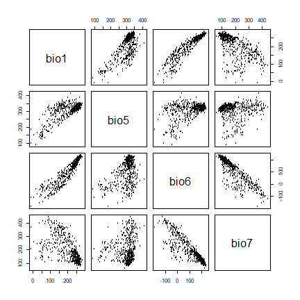
A pairs plot of the values of the climate data at the Bradypus occurrence sites.
To use the sdmdata and presvals in the next chapter, we save it
to disk.
saveRDS(sdmdata, "sdm.Rds")
saveRDS(presvals, "pvals.Rds")