Absence and background points
Some of the early species distribution model algorithms, such as Bioclim and Domain only use ‘presence’ data in the modeling process. Other methods also use ‘absence’ data or ‘background’ data. Logistic regression is the classical approach to analyzing presence and absence data (and it is still much used, often implemented in a generalized linear modeling (GLM) framework). If you have a large dataset with presence/absence from a well designed survey, you should use a method that can use these data (i.e. do not use a modeling method that only considers presence data). If you only have presence data, you can still use a method that needs absence data, by substituting absence data with background data.
Background data (e.g. Phillips et al. 2009) are not attempting to guess at absence locations, but rather to characterize environments in the study region. In this sense, background is the same, irrespective of where the species has been found. Background data establishes the environmental domain of the study, whilst presence data should establish under which conditions a species is more likely to be present than on average. A closely related but different concept, that of “pseudo-absences”, is also used for generating the non-presence class for logistic models. In this case, researchers sometimes try to guess where absences might occur – they may sample the whole region except at presence locations, or they might sample at places unlikely to be suitable for the species. We prefer the background concept because it requires fewer assumptions and has some coherent statistical methods for dealing with the “overlap” between presence and background points (e.g. Ward et al. 2009; Phillips and Elith, 2011).
Survey-absence data has value. In conjunction with presence records, it establishes where surveys have been done, and the prevalence of the species given the survey effort. That information is lacking for presence-only data, a fact that can cause substantial difficulties for modeling presence-only data well. However, absence data can also be biased and incomplete, as discussed in the literature on detectability (e.g., Kéry et al., 2010).
The terra package has a function to sample random points (background
data) from a study area. You can use a ‘mask’ to exclude area with no
data NA, e.g. areas not on land. You can use an ‘extent’ to further
restrict the area from which random locations are drawn.
In the example below, we first get the list of filenames with the
predictor raster data (discussed in detail in the next chapter). We use
a raster as a ‘mask’ in the randomPoints function such that the
background points are from the same geographic area, and only for places
where there are values (land, in our case).
Note that if the mask has the longitude/latitude coordinate reference
system, the spatSample method adjusts the probability of selecting a
cells according to cell area, which varies by latitude.
library(predicts)
## Loading required package: terra
## terra 1.9.21
# get the predictors filename
f1 <- system.file("ex/bio.tif", package="predicts")
f2 <- system.file("ex/biome.tif", package="predicts")
r <- rast(c(f1, f2))
# select 5000 random points
# set seed to assure that the examples will always
# have the same random sample.
set.seed(1963)
bg <- spatSample(r, 5000, "random", na.rm=TRUE, as.points=TRUE)
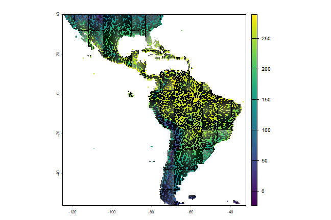
And inspect the results by plotting
plot(r, 1)
points(bg, cex=0.5)
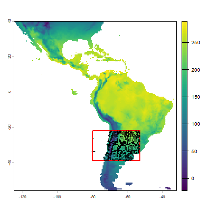
Now we repeat the sampling, but limit the area of sampling using a spatial extent
e <- ext(-80, -53, -39, -22)
bg2 <- spatSample(r, 500, "random", na.rm=TRUE, as.points=TRUE, ext=e)
plot(r, 1)
lines(e, col="red", lwd=2)
points(bg2, cex=0.5)
There are several approaches one could use to sample ‘pseudo-absence’
points, i.e., points from a more restricted area than ‘background’.
VanDerWal et al. (2009) sampled withn a radius of presence points. Here
is one way to implement that, using the Solanum acaule data.
We first read the cleaned and subsetted S. acaule data that we
produced in the previous chapter.
acfile <- file.path(system.file(package="predicts"), "ex/acaule.rds")
ac <- readRDS(acfile)
We first create a ‘circles’ model (see the chapter about geographic models), using an arbitrary radius of 50 km
# circles with a radius of 50 km
x <- buffer(ac, 50000)
pol <- aggregate(x)
And then we take a random sample of points within the polygons. We only want one point per grid cell.
# sample randomly from all circles
set.seed(999)
samp1 <- spatSample(pol, 500, "random")
We do not what to include the same raster cells multiple times
pcells <- cells(r, samp1)
# remote duplicates
pcells <- unique(pcells[,2])
# back to coordinates
xy <- xyFromCell(r, pcells)
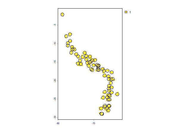
Plot to inspect the results:
plot(pol, axes=TRUE)
points(samp1, pch="+", cex=.5)
points(xy, cex=0.75, pch=20, col='blue')
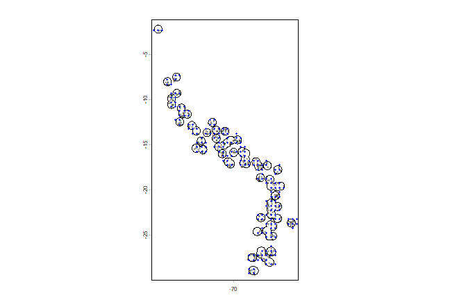
Note that the blue points are not all within the polygons (circles), as
they now represent the centers of the selected cells. We could choose to
select only those cells that have their centers within the circles,
using the intersect method.
spxy <- vect(xy, crs="+proj=longlat +datum=WGS84")
xyInside <- intersect(spxy, x)
Similar results could also be achieved via the raster functions
rasterize or extract.
# make a new, empty, smaller raster
m <- crop(rast(r[[1]]), ext(x)+1)
# extract cell numbers for the circles
v <- cells(m, x)
# get unique cell numbers from which you could sample
v <- unique(v[,"cell"])
head(v)
## [1] 1505 1541  918  919  954  955
# to display the results
m[v] <- 1
plot(m)
lines(x)