Raster data manipulation
Introduction
In this chapter general aspects of the design of the raster package
are discussed, notably the structure of the main classes, and what they
represent. The use of the package is illustrated in subsequent sections.
raster has a large number of functions, not all of them are
discussed here, and those that are discussed are mentioned only briefly.
See the help files of the package for more information on individual
functions and help("raster-package") for an index of functions by
topic.
Creating Raster* objects
A RasterLayer can easily be created from scratch using the function
raster. The default settings will create a global raster data
structure with a longitude/latitude coordinate reference system and 1 by
1 degree cells. You can change these settings by providing additional
arguments such as xmn, nrow, ncol, and/or crs, to the
function. You can also change these parameters after creating the
object. If you set the projection, this is only to properly define it,
not to change it. To transform a RasterLayer to another coordinate
reference system (projection) you can use the function 1projectRaster1.
Here is an example of creating and changing a RasterLayer object ‘r’
from scratch.
library(raster)
## Loading required package: sp
# RasterLayer with the default parameters
x <- raster()
x
## class      : RasterLayer
## dimensions : 180, 360, 64800  (nrow, ncol, ncell)
## resolution : 1, 1  (x, y)
## extent     : -180, 180, -90, 90  (xmin, xmax, ymin, ymax)
## crs        : +proj=longlat +datum=WGS84 +no_defs
With some other parameters
x <- raster(ncol=36, nrow=18, xmn=-1000, xmx=1000, ymn=-100, ymx=900)
These parameters can be changed. Resolution:
res(x)
## [1] 55.55556 55.55556
res(x) <- 100
res(x)
## [1] 100 100
Change the number of columns (this affects the resolution).
ncol(x)
## [1] 20
ncol(x) <- 18
ncol(x)
## [1] 18
res(x)
## [1] 111.1111 100.0000
Set the coordinate reference system (CRS) (i.e., define the projection).
projection(x) <- "+proj=utm +zone=48 +datum=WGS84"
x
## class      : RasterLayer
## dimensions : 10, 18, 180  (nrow, ncol, ncell)
## resolution : 111.1111, 100  (x, y)
## extent     : -1000, 1000, -100, 900  (xmin, xmax, ymin, ymax)
## crs        : +proj=utm +zone=48 +datum=WGS84 +units=m +no_defs
The objects x created in the examples above only consist of the
raster ‘geometry’, that is, we have defined the number of rows and
columns, and where the raster is located in geographic space, but there
are no cell-values associated with it. Setting and accessing values is
illustrated below.
First another example empty raster geometry.
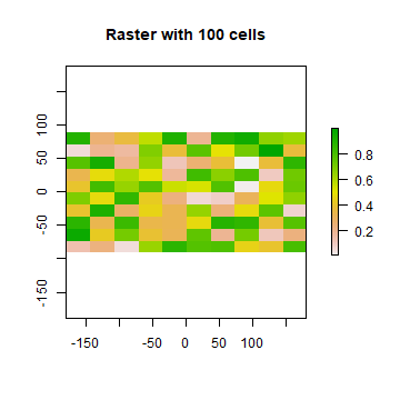
r <- raster(ncol=10, nrow=10)
ncell(r)
## [1] 100
hasValues(r)
## [1] FALSE
Use the ‘values’ function.
values(r) <- 1:ncell(r)
Another example.
set.seed(0)
values(r) <- runif(ncell(r))
hasValues(r)
## [1] TRUE
inMemory(r)
## [1] TRUE
values(r)[1:10]
##  [1] 0.8966972 0.2655087 0.3721239 0.5728534 0.9082078 0.2016819 0.8983897
##  [8] 0.9446753 0.6607978 0.6291140
plot(r, main='Raster with 100 cells')
In some cases, for example when you change the number of columns or
rows, you will lose the values associated with the RasterLayer if
there were any (or the link to a file if there was one). The same
applies, in most cases, if you change the resolution directly (as this
can affect the number of rows or columns). Values are not lost when
changing the extent as this change adjusts the resolution, but does not
change the number of rows or columns.
hasValues(r)
## [1] TRUE
res(r)
## [1] 36 18
dim(r)
## [1] 10 10  1
xmax(r)
## [1] 180
Now change the maximum x coordinate of the extent (bounding box) of the RasterLayer.
xmax(r) <- 0
hasValues(r)
## [1] TRUE
res(r)
## [1] 18 18
dim(r)
## [1] 10 10  1
And the number of columns (the values disappear)
ncol(r) <- 6
hasValues(r)
## [1] FALSE
res(r)
## [1] 30 18
dim(r)
## [1] 10  6  1
xmax(r)
## [1] 0
The function raster also allows you to create a RasterLayer from
another object, including another RasterLayer, RasterStack and
RasterBrick , as well as from a SpatialPixels* and
SpatialGrid* object (defined in the sp package), an Extent
object, a matrix, an im object (spatstat package), and others.
It is more common, however, to create a RasterLayer object from a
file. The raster package can use raster files in several formats,
including some ‘natively’ supported formats and other formats via the
rgdal package. Supported formats for reading include GeoTiff, ESRI,
ENVI, and ERDAS. Most formats supported for reading can also be written
to. Here is an example using the ‘Meuse’ dataset (taken from the sp
package), using a file in the native ‘raster-file’ format.
A notable feature of the raster package is that it can work with
raster datasets that are stored on disk and are too large to be loaded
into memory (RAM). The package can work with large files because the
objects it creates from these files only contain information about the
structure of the data, such as the number of rows and columns, the
spatial extent, and the filename, but it does not attempt to read all
the cell values in memory. In computations with these objects, data is
processed in chunks. If no output filename is specified to a function,
and the output raster is too large to keep in memory, the results are
written to a temporary file.
For this example, we first we get the name of an example file installed
with the package. Do not use this system.file construction of
your own files (just type the file name; don’t forget the forward
slashes).
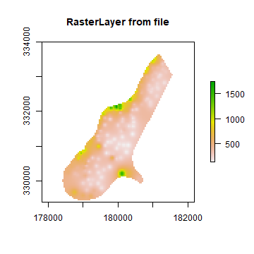
filename <- system.file("external/test.grd", package="raster")
filename
## [1] "C:/soft/R/R-devel/library/raster/external/test.grd"
r <- raster(filename)
filename(r)
## [1] "C:\\soft\\R\\R-devel\\library\\raster\\external\\test.grd"
hasValues(r)
## [1] TRUE
inMemory(r)
## [1] FALSE
plot(r, main='RasterLayer from file')
Multi-layer objects can be created in memory (from RasterLayer
objects) or from files.
Create three identical RasterLayer objects
r1 <- r2 <- r3 <- raster(nrow=10, ncol=10)
# Assign random cell values
values(r1) <- runif(ncell(r1))
values(r2) <- runif(ncell(r2))
values(r3) <- runif(ncell(r3))
Combine three RasterLayer objects into a RasterStack.
s <- stack(r1, r2, r3)
s
## class      : RasterStack
## dimensions : 10, 10, 100, 3  (nrow, ncol, ncell, nlayers)
## resolution : 36, 18  (x, y)
## extent     : -180, 180, -90, 90  (xmin, xmax, ymin, ymax)
## crs        : +proj=longlat +datum=WGS84 +no_defs
## names      :    layer.1,    layer.2,    layer.3
## min values : 0.01307758, 0.02778712, 0.06380247
## max values :  0.9926841,  0.9815635,  0.9960774
nlayers(s)
## [1] 3
Or combine the RasterLayer objects into a RasterBrick.
b1 <- brick(r1, r2, r3)
This is equivalent to:
b2 <- brick(s)
You can also create a RasterBrick from a file.
filename <- system.file("external/rlogo.grd", package="raster")
filename
## [1] "C:/soft/R/R-devel/library/raster/external/rlogo.grd"
b <- brick(filename)
b
## class      : RasterBrick
## dimensions : 77, 101, 7777, 3  (nrow, ncol, ncell, nlayers)
## resolution : 1, 1  (x, y)
## extent     : 0, 101, 0, 77  (xmin, xmax, ymin, ymax)
## crs        : +proj=merc +lon_0=0 +k=1 +x_0=0 +y_0=0 +datum=WGS84 +units=m +no_defs
## source     : rlogo.grd
## names      : red, green, blue
## min values :   0,     0,    0
## max values : 255,   255,  255
nlayers(b)
## [1] 3
Extract a single RasterLayer from a RasterBrick (or RasterStack).
r <- raster(b, layer=2)
In this case, that would be equivalent to creating it from disk with a
band=2 argument.
r <- raster(filename, band=2)
Raster algebra
Many generic functions that allow for simple and elegant raster algebra
have been implemented for Raster objects, including the normal
algebraic operators such as +, -, *, /, logical
operators such as >, >=, <, ==, ! and functions like
abs, round, ceiling, floor, trunc, sqrt,
log, log10, exp, cos, sin, atan, tan,
max, min, range, prod, sum, any, all. In
these functions you can mix raster objects with numbers, as long as
the first argument is a raster object.
Create an empty RasterLayer and assign values to cells.
r <- raster(ncol=10, nrow=10)
values(r) <- 1:ncell(r)
Now some algebra.
s <- r + 10
s <- sqrt(s)
s <- s * r + 5
r[] <- runif(ncell(r))
r <- round(r)
r <- r == 1
You can also use replacement functions.
s[r] <- -0.5
s[!r] <- 5
s[s == 5] <- 15
If you use multiple Raster objects (in functions where this is
relevant, such as range), these must have the same resolution and
origin. The origin of a Raster object is the point closest to (0, 0)
that you could get if you moved from a corners of a Raster object
toward that point in steps of the x and y resolution. Normally
these objects would also have the same extent, but if they do not, the
returned object covers the spatial intersection of the objects used.
When you use multiple multi-layer objects with different numbers or layers, the ‘shorter’ objects are ‘recycled’. For example, if you multiply a 4-layer object (a1, a2, a3, a4) with a 2-layer object (b1, b2), the result is a four-layer object (a1b1, a2b2, a3b1, a3b2).
r <- raster(ncol=5, nrow=5)
r[] <- 1
s <- stack(r, r+1)
q <- stack(r, r+2, r+4, r+6)
x <- r + s + q
x
## class      : RasterBrick
## dimensions : 5, 5, 25, 4  (nrow, ncol, ncell, nlayers)
## resolution : 72, 36  (x, y)
## extent     : -180, 180, -90, 90  (xmin, xmax, ymin, ymax)
## crs        : +proj=longlat +datum=WGS84 +no_defs
## source     : memory
## names      : layer.1, layer.2, layer.3, layer.4
## min values :       3,       6,       7,      10
## max values :       3,       6,       7,      10
Summary functions (min, max, mean, prod, sum, Median, cv, range, any,
all) always return a RasterLayer object. Perhaps this is not obvious
when using functions like min, sum or mean.
a <- mean(r,s,10)
b <- sum(r,s)
st <- stack(r, s, a, b)
sst <- sum(st)
sst
## class      : RasterLayer
## dimensions : 5, 5, 25  (nrow, ncol, ncell)
## resolution : 72, 36  (x, y)
## extent     : -180, 180, -90, 90  (xmin, xmax, ymin, ymax)
## crs        : +proj=longlat +datum=WGS84 +no_defs
## source     : memory
## names      : layer
## values     : 11.5, 11.5  (min, max)
Use cellStats if instead of a RasterLayer you want a single
number summarizing the cell values of each layer.
cellStats(st, 'sum')
## layer.1.1 layer.1.2 layer.2.1 layer.2.2   layer.3
##      25.0      25.0      50.0      87.5     100.0
cellStats(sst, 'sum')
## [1] 287.5
‘High-level’ functions
Several ‘high level’ functions have been implemented for RasterLayer
objects. ‘High level’ functions refer to functions that you would
normally find in a computer program that supports the analysis of raster
data. Here we briefly discuss some of these functions. All these
functions work for raster datasets that cannot be loaded into memory.
See the help files for more detailed descriptions of each function.
The high-level functions have some arguments in common. The first
argument is typically ‘x’ or ‘object’ and can be a RasterLayer, or,
in most cases, a RasterStack or RasterBrick. It is followed by
one or more arguments specific to the function (either additional
RasterLayer objects or other arguments), followed by a filename=””
and “…” arguments.
The default filename is an empty character “”. If you do not specify a
filename, the default action for the function is to return a raster
object that only exists in memory. However, if the function deems that
the raster object to be created would be too large to hold memory it
is written to a temporary file instead.
The “…” argument allows for setting additional arguments that are relevant when writing values to a file: the file format, datatype (e.g. integer or real values), and a to indicate whether existing files should be overwritten.
Modifying a Raster* object
There are several functions that deal with modifying the spatial extent
of Raster objects. The crop function lets you take a geographic
subset of a larger raster object. You can crop a Raster by
providing an extent object or another spatial object from which an
extent can be extracted (objects from classes deriving from Raster and
from Spatial in the sp package). An easy way to get an extent object is
to plot a RasterLayer and then use drawExtent to visually
determine the new extent (bounding box) to provide to the crop function.
trim crops a RasterLayer by removing the outer rows and columns
that only contain NA values. In contrast, extend adds new rows
and/or columns with NA values. The purpose of this could be to
create a new RasterLayer with the same Extent of another, larger,
RasterLayer such that they can be used together in other functions.
The merge function lets you merge 2 or more Raster objects into
a single new object. The input objects must have the same resolution and
origin (such that their cells neatly fit into a single larger raster).
If this is not the case you can first adjust one of the Raster
objects with use (dis)aggregate or resample.
aggregate and disaggregate allow for changing the resolution
(cell size) of a Raster object. In the case of aggregate, you
need to specify a function determining what to do with the grouped cell
values mean. It is possible to specify different (dis)aggregation
factors in the x and y direction. aggregate and disaggregate are
the best functions when adjusting cells size only, with an integer step
(e.g. each side 2 times smaller or larger), but in some cases that is
not possible.
For example, you may need nearly the same cell size, while shifting the
cell centers. In those cases, the resample function can be used. It
can do either nearest neighbor assignments (for categorical data) or
bilinear interpolation (for numerical data). Simple linear shifts of a
Raster object can be accomplished with the shift function or with
the extent function. resample should not be used to create a
Raster* object with much larger resolution. If such adjustments need to
be made then you can first use aggregate.
With the projectRaster function you can transform values of
Raster object to a new object with a different coordinate reference
system.
Here are some simple examples.
Aggregate and disaggregate.
r <- raster()
r[] <- 1:ncell(r)
ra <- aggregate(r, 20)
rd <- disaggregate(ra, 20)
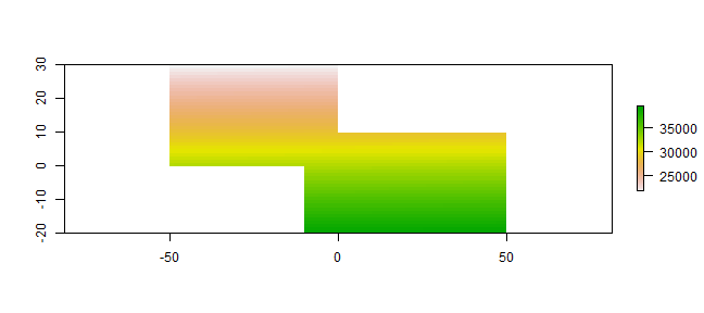
Crop and merge example.
r1 <- crop(r, extent(-50,0,0,30))
r2 <- crop(r, extent(-10,50,-20, 10))
m <- merge(r1, r2, filename='test.grd', overwrite=TRUE)
plot(m)
flip lets you flip the data (reverse order) in horizontal or
vertical direction – typically to correct for a ‘communication problem’
between different R packages or a misinterpreted file. rotate lets
you rotate longitude/latitude rasters that have longitudes from 0 to 360
degrees (often used by climatologists) to the standard -180 to 180
degrees system. With t you can rotate a Raster object 90
degrees.
Overlay
The overlay function can be used as an alternative to the raster
algebra discussed above. Overlay, like the functions discussed in the
following subsections provide either easy to use short-hand, or more
efficient computation for large (file based) objects.
With overlay you can combine multiple Raster objects (e.g. multiply
them). The related function mask removes all values from one layer
that are NA in another layer, and cover combines two layers by
taking the values of the first layer except where these are NA.
Calc
calc allows you to do a computation for a single raster object
by providing a function. If you supply a RasterLayer, another
RasterLayer is returned. If you provide a multi-layer object you get
a (single layer) RasterLayer if you use a summary type function
(e.g. sum but a RasterBrick if multiple layers are returned.
stackApply computes summary type layers for subsets of a
RasterStack or RasterBrick.
Reclassify
You can use cut or reclassify to replace ranges of values with
single values, or subs to substitute (replace) single values with
other values.
r <- raster(ncol=3, nrow=2)
r[] <- 1:ncell(r)
getValues(r)
## [1] 1 2 3 4 5 6
Set all values above 4 to NA
s <- calc(r, fun=function(x){ x[x < 4] <- NA; return(x)} )
as.matrix(s)
##      [,1] [,2] [,3]
## [1,]   NA   NA   NA
## [2,]    4    5    6
Divide the first raster with two times the square root of the second raster and add five.
w <- overlay(r, s, fun=function(x, y){ x / (2 * sqrt(y)) + 5 } )
as.matrix(w)
##      [,1]     [,2]     [,3]
## [1,]   NA       NA       NA
## [2,]    6 6.118034 6.224745
Remove from r all values that are NA in w.
u <- mask(r, w)
as.matrix(u)
##      [,1] [,2] [,3]
## [1,]   NA   NA   NA
## [2,]    4    5    6
Identify the cell values in u that are the same as in s.
v <- u==s
as.matrix(v)
##      [,1] [,2] [,3]
## [1,]   NA   NA   NA
## [2,] TRUE TRUE TRUE
Replace NA values in w with values of r.
cvr <- cover(w, r)
as.matrix(w)
##      [,1]     [,2]     [,3]
## [1,]   NA       NA       NA
## [2,]    6 6.118034 6.224745
Change value between 0 and 2 to 1, etc.
x <- reclassify(w, c(0,2,1,  2,5,2, 4,10,3))
as.matrix(x)
##      [,1] [,2] [,3]
## [1,]   NA   NA   NA
## [2,]    3    3    3
Substitute 2 with 40 and 3 with 50.
y <- subs(x, data.frame(id=c(2,3), v=c(40,50)))
as.matrix(y)
##      [,1] [,2] [,3]
## [1,]   NA   NA   NA
## [2,]   50   50   50
Focal functions
The focal function currently only work for (single layer)
RasterLayer objects. They make a computation using values in a
neighborhood of cells around a focal cell, and putting the result in the
focal cell of the output RasterLayer. The neighborhood is a user-defined
matrix of weights and could approximate any shape by giving some cells
zero weight. It is possible to only computes new values for cells that
are NA in the input RasterLayer.
Distance
There are a number of distance related functions. distance computes
the shortest distance to cells that are not NA. pointDistance
computes the shortest distance to any point in a set of points.
gridDistance computes the distance when following grid cells that
can be traversed (e.g. excluding water bodies). direction computes
the direction toward (or from) the nearest cell that is not NA.
adjacency determines which cells are adjacent to other cells. See
the gdistance package for more advanced distance calculations (cost
distance, resistance distance)
Spatial configuration
Function clump identifies groups of cells that are connected.
boundaries identifies edges, that is, transitions between cell
values. area computes the size of each grid cell (for unprojected
rasters), this may be useful to, e.g. compute the area covered by a
certain class on a longitude/latitude raster.
r <- raster(nrow=45, ncol=90)
r[] <- round(runif(ncell(r))*3)
a <- area(r)
zonal(a, r, 'sum')
##      zone       sum
## [1,]    0  93604336
## [2,]    1 168894837
## [3,]    2 158110025
## [4,]    3  87822040
Predictions
The package has two functions to make model predictions to (potentially
very large) rasters. predict takes a multilayer raster and a fitted
model as arguments. Fitted models can be of various classes, including
glm, gam, and RandomForest. The function interpolate is similar but
is for models that use coordinates as predictor variables, for example
in Kriging and spline interpolation.
Vector to raster conversion
The raster package supports point, line, and polygon to raster
conversion with the rasterize function. For vector type data
(points, lines, polygons), objects of Spatial* classes defined in the
sp package are used; but points can also be represented by a
two-column matrix (x and y).
Point to raster conversion is often done with the purpose to analyze the
point data. For example to count the number of distinct species
(represented by point observations) that occur in each raster cell.
rasterize takes a Raster object to set the spatial extent and
resolution, and a function to determine how to summarize the points (or
an attribute of each point) by cell.
Polygon to raster conversion is typically done to create a
RasterLayer that can act as a mask, i.e. to set to NA a set of
cells of a raster object, or to summarize values on a raster by
zone. For example a country polygon is transferred to a raster that is
then used to set all the cells outside that country to NA; whereas
polygons representing administrative regions such as states can be
transferred to a raster to summarize raster values by region.
It is also possible to convert the values of a RasterLayer to points
or polygons, using rasterToPoints and rasterToPolygons. Both
functions only return values for cells that are not NA. Unlike
rasterToPolygons, rasterToPoints is reasonably efficient and
allows you to provide a function to subset the output before it is
produced (which can be necessary for very large rasters as the point
object is created in memory).
Summarizing functions
When used with a Raster object as first argument, normal summary
statistics functions such as min, max and mean return a RasterLayer. You
can use cellStats if, instead, you want to obtain a summary for all
cells of a single Raster object. You can use freq to make a
frequency table, or to count the number of cells with a specified value.
Use zonal to summarize a Raster object using zones (areas with
the same integer number) defined in a RasterLayer and crosstab
to cross-tabulate two RasterLayer objects.
r <- raster(ncol=36, nrow=18)
r[] <- runif(ncell(r))
cellStats(r, mean)
## [1] 0.5179682
Zonal stats
s <- r
s[] <- round(runif(ncell(r)) * 5)
zonal(r, s, 'mean')
##      zone      mean
## [1,]    0 0.5144431
## [2,]    1 0.5480089
## [3,]    2 0.5249257
## [4,]    3 0.5194031
## [5,]    4 0.4853966
## [6,]    5 0.5218401
Count cells
freq(s)
##      value count
## [1,]     0    54
## [2,]     1   102
## [3,]     2   139
## [4,]     3   148
## [5,]     4   133
## [6,]     5    72
freq(s, value=3)
## [1] 148
Cross-tabulate
ctb <- crosstab(r*3, s)
head(ctb)
##        layer.2
## layer.1  0  1  2  3  4  5
##       0  8 13 21 16 24 10
##       1 17 31 42 56 45 24
##       2 19 31 52 54 37 27
##       3 10 27 24 22 27 11
Helper functions
The cell number is an important concept in the raster package. Raster
data can be thought of as a matrix, but in a RasterLayer it is more
commonly treated as a vector. Cells are numbered from the upper left
cell to the upper right cell and then continuing on the left side of the
next row, and so on until the last cell at the lower-right side of the
raster. There are several helper functions to determine the column or
row number from a cell and vice versa, and to determine the cell number
for x, y coordinates and vice versa.
library(raster)
r <- raster(ncol=36, nrow=18)
ncol(r)
## [1] 36
nrow(r)
## [1] 18
ncell(r)
## [1] 648
rowFromCell(r, 100)
## [1] 3
colFromCell(r, 100)
## [1] 28
cellFromRowCol(r,5,5)
## [1] 149
xyFromCell(r, 100)
##       x  y
## [1,] 95 65
cellFromXY(r, c(0,0))
## [1] 343
colFromX(r, 0)
## [1] 19
rowFromY(r, 0)
## [1] 10
Accessing cell values
Cell values can be accessed with several methods. Use getValues to
get all values or a single row; and getValuesBlock to read a block
(rectangle) of cell values.
r <- raster(system.file("external/test.grd", package="raster"))
v <- getValues(r, 50)
v[35:39]
## [1] 743.8288 706.2302 646.0078 686.7291 758.0649
getValuesBlock(r, 50, 1, 35, 5)
## [1] 743.8288 706.2302 646.0078 686.7291 758.0649
You can also read values using cell numbers or coordinates (xy) using
the extract method.
cells <- cellFromRowCol(r, 50, 35:39)
cells
## [1] 3955 3956 3957 3958 3959
extract(r, cells)
## [1] 743.8288 706.2302 646.0078 686.7291 758.0649
xy <- xyFromCell(r, cells)
xy
##           x      y
## [1,] 179780 332020
## [2,] 179820 332020
## [3,] 179860 332020
## [4,] 179900 332020
## [5,] 179940 332020
extract(r, xy)
## [1] 743.8288 706.2302 646.0078 686.7291 758.0649
You can also extract values using SpatialPolygons* or
SpatialLines*. The default approach for extracting raster values
with polygons is that a polygon has to cover the center of a cell, for
the cell to be included. However, you can use argument “weights=TRUE” in
which case you get, apart from the cell values, the percentage of each
cell that is covered by the polygon, so that you can apply, e.g., a “50%
area covered” threshold, or compute an area-weighted average.
In the case of lines, any cell that is crossed by a line is included. For lines and points, a cell that is only ‘touched’ is included when it is below or to the right (or both) of the line segment/point (except for the bottom row and right-most column).
In addition, you can use standard R indexing to access values, or to
replace values (assign new values to cells) in a raster object. If
you replace a value in a raster object based on a file, the
connection to that file is lost (because it now is different from that
file). Setting raster values for very large files will be very slow with
this approach as each time a new (temporary) file, with all the values,
is written to disk. If you want to overwrite values in an existing file,
you can use update (with caution!)
r[cells]
## [1] 743.8288 706.2302 646.0078 686.7291 758.0649
r[1:4]
## [1] NA NA NA NA
filename(r)
## [1] "C:\\soft\\R\\R-devel\\library\\raster\\external\\test.grd"
r[2:3] <- 10
r[1:4]
## [1] NA 10 10 NA
filename(r)
## [1] ""
Note that in the above examples values are retrieved using cell numbers. That is, a raster is represented as a (one-dimensional) vector. Values can also be inspected using a (two-dimensional) matrix notation. As for R matrices, the first index represents the row number, the second the column number.
r[1]
## [1] NA
r[2,2]
## [1] NA
r[1,]
##  [1] NA 10 10 NA NA NA NA NA NA NA NA NA NA NA NA NA NA NA NA NA NA NA NA NA NA
## [26] NA NA NA NA NA NA NA NA NA NA NA NA NA NA NA NA NA NA NA NA NA NA NA NA NA
## [51] NA NA NA NA NA NA NA NA NA NA NA NA NA NA NA NA NA NA NA NA NA NA NA NA NA
## [76] NA NA NA NA NA
r[,2]
##   [1]  10.0000       NA       NA       NA       NA       NA       NA       NA
##   [9]       NA       NA       NA       NA       NA       NA       NA       NA
##  [17]       NA       NA       NA       NA       NA       NA       NA       NA
##  [25]       NA       NA       NA       NA       NA       NA       NA       NA
##  [33]       NA       NA       NA       NA       NA       NA       NA       NA
##  [41]       NA       NA       NA       NA       NA       NA       NA       NA
##  [49]       NA       NA       NA       NA       NA       NA       NA       NA
##  [57]       NA       NA       NA       NA       NA       NA       NA       NA
##  [65]       NA       NA       NA       NA       NA       NA       NA       NA
##  [73]       NA       NA       NA       NA       NA       NA       NA       NA
##  [81]       NA       NA       NA       NA       NA       NA       NA       NA
##  [89]       NA       NA       NA       NA 509.6615 504.0837 495.6735 486.9267
##  [97] 479.6082 474.3188 471.4189 469.5895 468.7051 469.8029 472.0836 474.1420
## [105]       NA       NA       NA       NA       NA       NA       NA       NA
## [113]       NA       NA       NA
r[1:3,1:3]
## [1] NA 10 10 NA NA NA NA NA NA
# keep the matrix structure
r[1:3,1:3, drop=FALSE]
## class      : RasterLayer
## dimensions : 3, 3, 9  (nrow, ncol, ncell)
## resolution : 40, 40  (x, y)
## extent     : 178400, 178520, 333880, 334000  (xmin, xmax, ymin, ymax)
## crs        : +proj=sterea +lat_0=52.1561605555556 +lon_0=5.38763888888889 +k=0.9999079 +x_0=155000 +y_0=463000 +datum=WGS84 +units=m +no_defs
## source     : memory
## names      : layer
## values     : 10, 10  (min, max)
Accessing values through this type of indexing should be avoided inside
functions as it is less efficient than accessing values via functions
like getValues.
Coercion to other classes
Although the raster package defines its own set of classes, it is
easy to coerce objects of these classes to objects of the Spatial
family defined in the sp package. This allows for using functions
defined by sp (e.g. spplot) and for using other packages that expect
Spatial* objects. To create a Raster object from variable n in a
SpatialGrid* x use raster(x, n) or stack(x) or brick(x).
Vice versa use as( , ). You can also convert objects of class im
(spatstat) and others to a RasterLayer using the raster,
stack or brick functions.
r1 <- raster(ncol=36, nrow=18)
r2 <- r1
r1[] <- runif(ncell(r1))
r2[] <- runif(ncell(r1))
s <- stack(r1, r2)
sgdf <- as(s, 'SpatialGridDataFrame')
newr2 <- raster(sgdf, 2)
news <- stack(sgdf)