Spatial data

Introduction

Spatial phenomena can generally be thought of as either discrete objects with clear boundaries or as a continuous phenomenon that can be observed everywhere, but does not have natural boundaries. Discrete spatial objects may refer to a river, road, country, town, or a research site. Examples of continuous phenomena, or “spatial fields”, include elevation, temperature, and air quality.

Spatial objects are usually represented by vector data. Such data consists of a description of the “geometry” or “shape” of the objects, and normally also includes additional variables. For example, a vector data set may describe the borders of the countries of the world (geometry), and also store their names and the size of their population in 2015; or the geometry of the roads in an area, as well as their type and names. These additional variables are often referred to as “attributes”. Continuous spatial data (fields) are usually represented with a raster data structure. We discuss these two data types in turn.

Vector data

The main vector data types are points, lines and polygons. In all cases, the geometry of these data structures consists of sets of coordinate pairs (x, y). Points are the simplest case. Each point has one coordinate pair, and n associated variables. For example, a point might represent a place where a rat was trapped, and the attributes could include the date it was captured, the person who captured it, the species size and sex, and information about the habitat. It is also possible to combine several points into a multi-point structure, with a single attribute record. For example, all the coffee shops in a town could be considered as a single geometry.

The geometry of lines is a just a little bit more complex. First note that in this context, the term ‘line’ refers to a set of one or more polylines (connected series of line segments). For example, in spatial analysis, a river and all its tributaries could be considered as a single ‘line’ (but they could also also be several lines, perhaps one for each tributary river). Lines are represented as ordered sets of coordinates (nodes). The actual line segments can be computed (and drawn on a map) by connecting the points. Thus, the representation of a line is very similar to that of a multi-point structure. The main difference is that the ordering of the points is important, because we need to know which points should be connected. A network (e.g. a road or river network), or spatial graph, is a special type of lines geometry where there is additional information about things like flow, connectivity, direction, and distance.

A polygon refers to a set of closed polylines. The geometry is very similar to that of lines, but to close a polygon the last coordinate pair coincides with the first pair. A complication with polygons is that they can have holes (that is a polygon entirely enclosed by another polygon, that serves to remove parts of the enclosing polygon (for example to show an island inside a lake. Also, valid polygons do not self-intersect (but it is OK for a line to self-cross). Again, multiple polygons can be considered as a single geometry. For example, Indonesia consists of many islands. Each island can be represented by a single polygon, but together then can be represent a single (multi-) polygon representing the entire country.

Raster data

Raster data is commonly used to represent spatially continuous phenomena such as elevation. A raster divides the world into a grid of equally sized rectangles (referred to as cells or, in the context of satellite remote sensing, pixels) that all have one or more values (or missing values) for the variables of interest. A raster cell value should normally represent the average (or majority) value for the area it covers. However, in some cases the values are actually estimates for the center of the cell (in essence becoming a regular set of points with an attribute).

In contrast to vector data, in raster data the geometry is not explicitly stored as coordinates. It is implicitly set by knowing the spatial extent and the number or rows and columns in which the area is divided. From the extent and number of rows and columns, the size of the raster cells (spatial resolution) can be computed. While raster cells can be thought of as a set of regular polygons, it would be very inefficient to represent the data that way as coordinates for each cell would have to be stored explicitly. It would also dramatically increase processing speed in most cases.

Continuous surface data are sometimes stored as triangulated irregular networks (TINs); these are not discussed here.

Simple representation of spatial data

The basic data types in R are numbers, characters, logical (TRUE or FALSE) and factor values. Values of a single type can be combined in vectors and matrices, and variables of multiple types can be combined into a data.frame. We can represent (only very) basic spatial data with these data types. Let’s say we have the location (represented by longitude and latitude) of ten weather stations (named A to J) and their annual precipitation.

In the example below we make a very simple map. Note that a map is special type of plot (like a scatter plot, barplot, etc.). A map is a plot of geospatial data that also has labels and other graphical objects such as a scale bar or legend. The spatial data itself should not be referred to as a map.

name <- LETTERS[1:10]
longitude <- c(-116.7, -120.4, -116.7, -113.5, -115.5,
               -120.8, -119.5, -113.7, -113.7, -110.7)
latitude <- c(45.3, 42.6, 38.9, 42.1, 35.7, 38.9,
              36.2, 39, 41.6, 36.9)
stations <- cbind(longitude, latitude)
# Simulated rainfall data
set.seed(0)
precip <- round((runif(length(latitude))*10)^3)

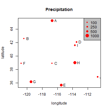
A map of point locations is not that different from a basic x-y scatter plot. Here I make a plot (a map in this case) that shows the location of the weather stations, and the size of the dots is proportional to the amount of precipitation. The point size is set with argument cex.

psize <- 1 + precip/500
plot(stations, cex=psize, pch=20, col='red', main='Precipitation')
# add names to plot
text(stations, name, pos=4)
# add a legend
breaks <- c(100, 250, 500, 1000)
legend.psize <- 1+breaks/500
legend("topright", legend=breaks, pch=20, pt.cex=legend.psize, col='red', bg='gray')

Note that the data are represented by “longitude, latitude”, in that order, do not use “latitude, longitude” because on most maps latitude (North/South) is used for the vertical axis and longitude (East/West) for the horizontal axis. This is important to keep in mind, as it is a very common source of mistakes!

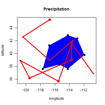
We can add multiple sets of points to the plot, and even draw lines and polygons:

lon <- c(-116.8, -114.2, -112.9, -111.9, -114.2, -115.4, -117.7)
lat <- c(41.3, 42.9, 42.4, 39.8, 37.6, 38.3, 37.6)
x <- cbind(lon, lat)
plot(stations, main='Precipitation')
polygon(x, col='blue', border='light blue')
lines(stations, lwd=3, col='red')
points(x, cex=2, pch=20)
points(stations, cex=psize, pch=20, col='red', main='Precipitation')

The above illustrates how numeric vectors representing locations can be used to draw simple maps. It also shows how points can (and typically are) represented by pairs of numbers. A line and a polygon can be represented by a number of these points. Polygons need to “closed”, that is, the first point must coincide with the last point, but the polygon function took care of that for us.

There are cases where a simple approach like this may suffice and you may come across this in older R code or packages. Likewise, raster data could be represented by a matrix or higher-order array. Particularly when only dealing with point data such an approach may be practical. For example, a spatial data set representing points and attributes could be made by combining geometry and attributes in a single ’data.frame`.

wst <- data.frame(longitude, latitude, name, precip)
wst
##    longitude latitude name precip
## 1     -116.7     45.3    A    721
## 2     -120.4     42.6    B     19
## 3     -116.7     38.9    C     52
## 4     -113.5     42.1    D    188
## 5     -115.5     35.7    E    749
## 6     -120.8     38.9    F      8
## 7     -119.5     36.2    G    725
## 8     -113.7     39.0    H    843
## 9     -113.7     41.6    I    289
## 10    -110.7     36.9    J    249

However, wst is a data.frame and R does not automatically understand the special meaning of the first two columns, or to what coordinate reference system it refers (longitude/latitude, or perhaps UTM zone 17S, or ….?).

Moreover, it is non-trivial to do some basic spatial operations. For example, the blue polygon drawn on the map above might represent a state, and a next question might be which of the 10 stations fall within that polygon. And how about any other operation on spatial data, including reading from and writing data to files? To facilitate such operation a number of R packages have been developed that define new spatial data types that can be used for this type of specialized operations. The most important packages that define such spatial data structures are sp and raster. These data types are discussed in the next chapters.