Vector data manipulation
Example SpatialPolygons
f <- system.file("external/lux.shp", package="raster")
library(raster)
p <- shapefile(f)
p
## class : SpatialPolygonsDataFrame
## features : 12
## extent : 5.74414, 6.528252, 49.44781, 50.18162 (xmin, xmax, ymin, ymax)
## crs : +proj=longlat +datum=WGS84 +no_defs
## variables : 5
## names : ID_1, NAME_1, ID_2, NAME_2, AREA
## min values : 1, Diekirch, 1, Capellen, 76
## max values : 3, Luxembourg, 12, Wiltz, 312
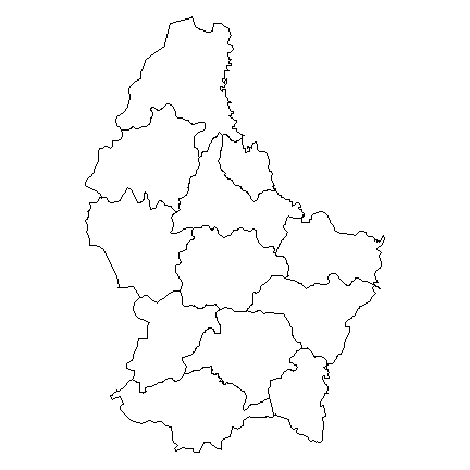
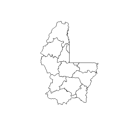
par(mai=c(0,0,0,0))
plot(p)
Basics
Basic operations are pretty much like working with a data.frame.
Geometry and attributes
To extract the attributes (data.frame) from a Spatial object, use:
d <- data.frame(p)
head(d)
##   ID_1       NAME_1 ID_2     NAME_2 AREA
## 0    1     Diekirch    1   Clervaux  312
## 1    1     Diekirch    2   Diekirch  218
## 2    1     Diekirch    3    Redange  259
## 3    1     Diekirch    4    Vianden   76
## 4    1     Diekirch    5      Wiltz  263
## 5    2 Grevenmacher    6 Echternach  188
Extracting geometry (rarely needed).
g <- geom(p)
head(g)
##      object part cump hole        x        y
## [1,]      1    1    1    0 6.026519 50.17767
## [2,]      1    1    1    0 6.031361 50.16563
## [3,]      1    1    1    0 6.035646 50.16410
## [4,]      1    1    1    0 6.042747 50.16157
## [5,]      1    1    1    0 6.043894 50.16116
## [6,]      1    1    1    0 6.048243 50.16008
Variables
Extracting a variable.
p$NAME_2
##  [1] "Clervaux"         "Diekirch"         "Redange"          "Vianden"
##  [5] "Wiltz"            "Echternach"       "Remich"           "Grevenmacher"
##  [9] "Capellen"         "Esch-sur-Alzette" "Luxembourg"       "Mersch"
Sub-setting by variable. Note how this is different from the above example. Above a vector of values is returned. With the approach below you get a new SpatialPolygonsDataFrame with only one variable.
p[, 'NAME_2']
## class       : SpatialPolygonsDataFrame
## features    : 12
## extent      : 5.74414, 6.528252, 49.44781, 50.18162  (xmin, xmax, ymin, ymax)
## crs         : +proj=longlat +datum=WGS84 +no_defs
## variables   : 1
## names       :   NAME_2
## min values  : Capellen
## max values  :    Wiltz
Adding a new variable.
set.seed(0)
p$new <- sample(letters, length(p))
p
## class       : SpatialPolygonsDataFrame
## features    : 12
## extent      : 5.74414, 6.528252, 49.44781, 50.18162  (xmin, xmax, ymin, ymax)
## crs         : +proj=longlat +datum=WGS84 +no_defs
## variables   : 6
## names       : ID_1,     NAME_1, ID_2,   NAME_2, AREA, new
## min values  :    1,   Diekirch,    1, Capellen,   76,   a
## max values  :    3, Luxembourg,   12,    Wiltz,  312,   z
Assigning a new value to an existing variable.
p$new <- sample(LETTERS, length(p))
p
## class       : SpatialPolygonsDataFrame
## features    : 12
## extent      : 5.74414, 6.528252, 49.44781, 50.18162  (xmin, xmax, ymin, ymax)
## crs         : +proj=longlat +datum=WGS84 +no_defs
## variables   : 6
## names       : ID_1,     NAME_1, ID_2,   NAME_2, AREA, new
## min values  :    1,   Diekirch,    1, Capellen,   76,   E
## max values  :    3, Luxembourg,   12,    Wiltz,  312,   Z
To get rid of a variable.
p$new <- NULL
Merge
You can join a table (data.frame) with a Spatial* object with
merge.
dfr <- data.frame(District=p$NAME_1, Canton=p$NAME_2, Value=round(runif(length(p), 100, 1000)))
dfr <- dfr[order(dfr$Canton), ]
pm <- merge(p, dfr, by.x=c('NAME_1', 'NAME_2'), by.y=c('District', 'Canton'))
pm
## class       : SpatialPolygonsDataFrame
## features    : 12
## extent      : 5.74414, 6.528252, 49.44781, 50.18162  (xmin, xmax, ymin, ymax)
## crs         : +proj=longlat +datum=WGS84 +no_defs
## variables   : 6
## names       :     NAME_1,   NAME_2, ID_1, ID_2, AREA, Value
## min values  :   Diekirch, Capellen,    1,    1,   76,   197
## max values  : Luxembourg,    Wiltz,    3,   12,  312,   845
Records
Selecting rows (records).
i <- which(p$NAME_1 == 'Grevenmacher')
g <- p[i,]
g
## class       : SpatialPolygonsDataFrame
## features    : 3
## extent      : 6.169137, 6.528252, 49.46498, 49.85403  (xmin, xmax, ymin, ymax)
## crs         : +proj=longlat +datum=WGS84 +no_defs
## variables   : 5
## names       : ID_1,       NAME_1, ID_2,     NAME_2, AREA
## min values  :    2, Grevenmacher,    6, Echternach,  129
## max values  :    2, Grevenmacher,   12,     Remich,  210
It is also possible to interactively select and query records by
clicking on a plotted dataset. That is difficult to show here. See
?select for interactively selecting spatial features and ?click
to identify attributes by clicking on a plot (map).
Append and aggregate
Append
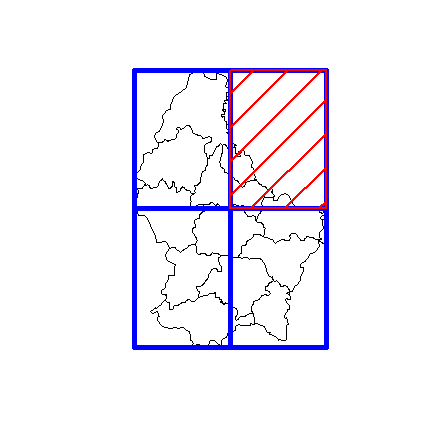
More example data. Object z, consisting of four polygons, and z2
which is one of these four polygons.
z <- raster(p, nrow=2, ncol=2, vals=1:4)
names(z) <- 'Zone'
# coerce RasterLayer to SpatialPolygonsDataFrame
z <- as(z, 'SpatialPolygonsDataFrame')
z
## class       : SpatialPolygonsDataFrame
## features    : 4
## extent      : 5.74414, 6.528252, 49.44781, 50.18162  (xmin, xmax, ymin, ymax)
## crs         : +proj=longlat +datum=WGS84 +no_defs
## variables   : 1
## names       : Zone
## min values  :    1
## max values  :    4
z2 <- z[2,]
plot(p)
plot(z, add=TRUE, border='blue', lwd=5)
plot(z2, add=TRUE, border='red', lwd=2, density=3, col='red')
To append Spatial* objects of the same (vector) type you can use
bind
b <- bind(p, z)
head(b)
##   ID_1       NAME_1 ID_2     NAME_2 AREA Zone
## 1    1     Diekirch    1   Clervaux  312   NA
## 2    1     Diekirch    2   Diekirch  218   NA
## 3    1     Diekirch    3    Redange  259   NA
## 4    1     Diekirch    4    Vianden   76   NA
## 5    1     Diekirch    5      Wiltz  263   NA
## 6    2 Grevenmacher    6 Echternach  188   NA
tail(b)
##    ID_1     NAME_1 ID_2     NAME_2 AREA Zone
## 11    3 Luxembourg   10 Luxembourg  237   NA
## 12    3 Luxembourg   11     Mersch  233   NA
## 13   NA       <NA>   NA       <NA>   NA    1
## 14   NA       <NA>   NA       <NA>   NA    2
## 15   NA       <NA>   NA       <NA>   NA    3
## 16   NA       <NA>   NA       <NA>   NA    4
Note how bind allows you to append Spatial* objects with
different attribute names.
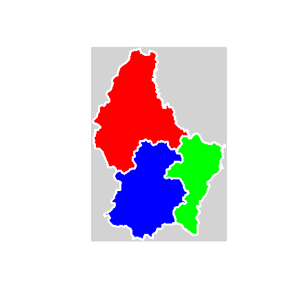
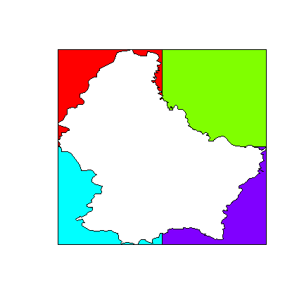
Aggregate
pa <- aggregate(p, by='NAME_1')
za <- aggregate(z)
plot(za, col='light gray', border='light gray', lwd=5)
plot(pa, add=TRUE, col=rainbow(3), lwd=3, border='white')
You can also aggregate by providing a second Spatial object (see
?sp::aggregate)
Aggregate without dissolve
zag <- aggregate(z, dissolve=FALSE)
zag
## class       : SpatialPolygons
## features    : 1
## extent      : 5.74414, 6.528252, 49.44781, 50.18162  (xmin, xmax, ymin, ymax)
## crs         : +proj=longlat +datum=WGS84 +no_defs
plot(zag, col="light gray")
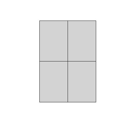
This is a structure that is similar to what you may get for an
archipelago: multiple polygons represented as one entity (one row). Use
disaggregate to split these up into their parts.
zd <- disaggregate(zag)
zd
## class       : SpatialPolygons
## features    : 4
## extent      : 5.74414, 6.528252, 49.44781, 50.18162  (xmin, xmax, ymin, ymax)
## crs         : +proj=longlat +datum=WGS84 +no_defs
Overlay
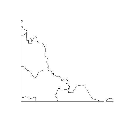
Erase
Erase a part of a SpatialPolygons object
e <- erase(p, z2)
This is equivalent to
e <- p - z2
plot(e)
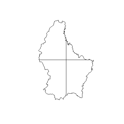
Intersect
Intersect SpatialPolygons
i <- intersect(p, z2)
plot(i)
This is equivalent to
i <- p * z2
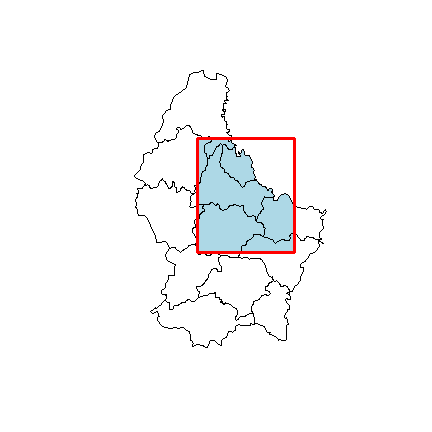
You can also intersect with an Extent (rectangle).
e <- extent(6, 6.4, 49.7, 50)
pe <- crop(p, e)
plot(p)
plot(pe, col='light blue', add=TRUE)
plot(e, add=TRUE, lwd=3, col='red')
Union
Get the union of two SpatialPolygon* objects.
u <- union(p, z)
This is equivalent to
u <- p + z
Note that there are many more polygons now. One for each unique combination of polygons (and attributes in this case).
u
## class       : SpatialPolygonsDataFrame
## features    : 28
## extent      : 5.74414, 6.528252, 49.44781, 50.18162  (xmin, xmax, ymin, ymax)
## crs         : +proj=longlat +datum=WGS84 +no_defs
## variables   : 6
## names       : Zone, ID_1,     NAME_1, ID_2,   NAME_2, AREA
## min values  :    1,    1,   Diekirch,    1, Capellen,   76
## max values  :    4,    3, Luxembourg,   12,    Wiltz,  312
set.seed(5)
plot(u, col=sample(rainbow(length(u))))

Cover
Cover is a combination of intersect and union
cov <- cover(p, z)
cov
## class       : SpatialPolygonsDataFrame
## features    : 6
## extent      : 5.74414, 6.528252, 49.44781, 50.18162  (xmin, xmax, ymin, ymax)
## crs         : +proj=longlat +datum=WGS84 +no_defs
## variables   : 6
## names       : ID_1,       NAME_1, ID_2,     NAME_2, AREA, Zone
## min values  :    1,     Diekirch,    1,   Clervaux,  188,    1
## max values  :    2, Grevenmacher,    6, Echternach,  312,    4
plot(cov)
Difference
The symmetrical difference of two SpatialPolygons* objects
dif <- symdif(z,p)
plot(dif, col=rainbow(length(dif)))
dif
## class       : SpatialPolygonsDataFrame
## features    : 4
## extent      : 5.74414, 6.528252, 49.44781, 50.18162  (xmin, xmax, ymin, ymax)
## crs         : NA
## variables   : 1
## names       : Zone
## min values  :    1
## max values  :    4
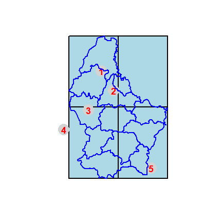
Spatial queries
Query polygons with points.
pts <- matrix(c(6, 6.1, 5.9, 5.7, 6.4, 50, 49.9, 49.8, 49.7, 49.5), ncol=2)
spts <- SpatialPoints(pts, proj4string=crs(p))
plot(z, col='light blue', lwd=2)
points(spts, col='light gray', pch=20, cex=6)
text(spts, 1:nrow(pts), col='red', font=2, cex=1.5)
lines(p, col='blue', lwd=2)
Use over for queries between Spatial* objects
over(spts, p)
##   ID_1   NAME_1 ID_2   NAME_2 AREA
## 1    1 Diekirch    5    Wiltz  263
## 2    1 Diekirch    2 Diekirch  218
## 3    1 Diekirch    3  Redange  259
## 4   NA     <NA>   NA     <NA>   NA
## 5   NA     <NA>   NA     <NA>   NA
over(spts, z)
##   Zone
## 1    1
## 2    1
## 3    3
## 4   NA
## 5    4
extract is generally used for queries between Spatial* and Raster*
objects, but it can also be used here.
extract(z, pts)
##   point.ID poly.ID Zone
## 1        1       1    1
## 2        2       1    1
## 3        3       3    3
## 4        4      NA   NA
## 5        5       4    4