Raster data
Introduction
The sp package supports raster (gridded) data with with the
SpatialGridDataFrame and SpatialPixelsDataFrame classes.
However, we will focus on classes from the raster package for raster
data. The raster package is built around a number of classes of which
the RasterLayer, RasterBrick, and RasterStack classes are
the most important. When discussing methods that can operate on all
three of these objects, they are referred to as ’Raster*’ objects.
The raster package has functions for creating, reading,
manipulating, and writing raster data. The package provides, among other
things, general raster data manipulation functions that can easily be
used to develop more specific functions. For example, there are
functions to read a chunk of raster values from a file or to convert
cell numbers to coordinates and back. The package also implements raster
algebra and many other functions for raster data manipulation.
RasterLayer
A RasterLayer object represents single-layer (variable) raster data.
A RasterLayer object always stores a number of fundamental
parameters that describe it. These include the number of columns and
rows, the spatial extent, and the Coordinate Reference System. In
addition, a RasterLayer can store information about the file in
which the raster cell values are stored (if there is such a file). A
RasterLayer can also hold the raster cell values in memory.
Here I create a RasterLayer from scratch. But note that in most
cases where real data is analyzed, these objects are created from a
file.
library(raster)
r <- raster(ncol=10, nrow=10, xmx=-80, xmn=-150, ymn=20, ymx=60)
r
## class      : RasterLayer
## dimensions : 10, 10, 100  (nrow, ncol, ncell)
## resolution : 7, 4  (x, y)
## extent     : -150, -80, 20, 60  (xmin, xmax, ymin, ymax)
## crs        : +proj=longlat +datum=WGS84 +no_defs
Object r only has the skeleton of a raster data set. That is, it
knows about its location, resolution, etc., but there are no values
associated with it. Let’s assign some values. In this case I assign a
vector of random numbers with a length that is equal to the number of
cells of the RasterLayer.
values(r) <- runif(ncell(r))
r
## class      : RasterLayer
## dimensions : 10, 10, 100  (nrow, ncol, ncell)
## resolution : 7, 4  (x, y)
## extent     : -150, -80, 20, 60  (xmin, xmax, ymin, ymax)
## crs        : +proj=longlat +datum=WGS84 +no_defs
## source     : memory
## names      : layer
## values     : 0.01307758, 0.9926841  (min, max)
You can also assign cell numbers (in this case overwriting the previous values)
values(r) <- 1:ncell(r)
r
## class      : RasterLayer
## dimensions : 10, 10, 100  (nrow, ncol, ncell)
## resolution : 7, 4  (x, y)
## extent     : -150, -80, 20, 60  (xmin, xmax, ymin, ymax)
## crs        : +proj=longlat +datum=WGS84 +no_defs
## source     : memory
## names      : layer
## values     : 1, 100  (min, max)
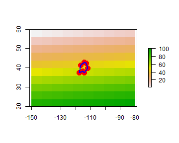
We can plot this object.
plot(r)
# add polygon and points
lon <- c(-116.8, -114.2, -112.9, -111.9, -114.2, -115.4, -117.7)
lat <- c(41.3, 42.9, 42.4, 39.8, 37.6, 38.3, 37.6)
lonlat <- cbind(lon, lat)
pols <- spPolygons(lonlat, crs='+proj=longlat +datum=WGS84')
points(lonlat, col='red', pch=20, cex=3)
plot(pols, border='blue', lwd=2, add=TRUE)
RasterStack and RasterBrick
It is quite common to analyze raster data using single-layer objects.
However, in many cases multi-variable raster data sets are used. The
raster package has two classes for multi-layer data the
RasterStack and the RasterBrick. The principal difference
between these two classes is that a RasterBrick can only be linked
to a single (multi-layer) file. In contrast, a RasterStack can be
formed from separate files and/or from a few layers (‘bands’) from a
single file.
In fact, a RasterStack is a collection of RasterLayer objects
with the same spatial extent and resolution. In essence it is a list of
RasterLayer objects. A RasterStack can easily be formed form a
collection of files in different locations and these can be mixed with
RasterLayer objects that only exist in the RAM memory (not on disk).
A RasterBrick is truly a multi-layered object, and processing a
RasterBrick can be more efficient than processing a RasterStack
representing the same data. However, it can only refer to a single file.
A typical example of such a file would be a multi-band satellite image
or the output of a global climate model (with e.g., a time series of
temperature values for each day of the year for each raster cell).
Methods that operate on RasterStack and RasterBrick objects
typically return a RasterBrick object.
Thus, the main difference is that a RasterStack is loose collection
of RasterLayer objects that can refer to different files (but must
all have the same extent and resolution), whereas a RasterBrick can
only point to a single file.
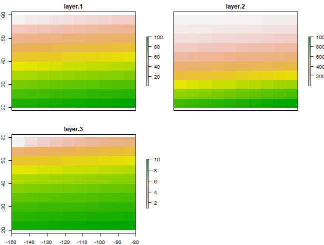
Here is an example how you can make a RasterStack from multiple layers.
r2 <- r * r
r3  <- sqrt(r)
s <- stack(r, r2, r3)
s
## class      : RasterStack
## dimensions : 10, 10, 100, 3  (nrow, ncol, ncell, nlayers)
## resolution : 7, 4  (x, y)
## extent     : -150, -80, 20, 60  (xmin, xmax, ymin, ymax)
## crs        : +proj=longlat +datum=WGS84 +no_defs
## names      : layer.1, layer.2, layer.3
## min values :       1,       1,       1
## max values :     100,   10000,      10
plot(s)
And you can make a RasterBrick from a RasterStack.
b <- brick(s)
b
## class      : RasterBrick
## dimensions : 10, 10, 100, 3  (nrow, ncol, ncell, nlayers)
## resolution : 7, 4  (x, y)
## extent     : -150, -80, 20, 60  (xmin, xmax, ymin, ymax)
## crs        : +proj=longlat +datum=WGS84 +no_defs
## source     : memory
## names      : layer.1, layer.2, layer.3
## min values :       1,       1,       1
## max values :     100,   10000,      10