Kriging
Alberta Rainfall
Recreating Figures 10.2, 10.13 & 10.14 in O’Sullivan and Unwin (2010).
We need the rspatial packge to get the data we will use.
if (!require("rspatial")) remotes::install_github('rspatial/rspatial')
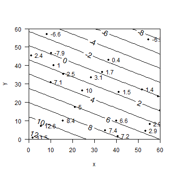
Figure 10.2
library(rspatial)
a <- sp_data('alberta.csv')
m <- lm(z ~ x + y, data=a)
summary(m)
##
## Call:
## lm(formula = z ~ x + y, data = a)
##
## Residuals:
##    Min     1Q Median     3Q    Max
## -7.763 -1.143 -0.081  1.520  6.600
##
## Coefficients:
##             Estimate Std. Error t value Pr(>|t|)
## (Intercept) 13.16438    1.55646   8.458 3.34e-08 ***
## x           -0.11983    0.03163  -3.788  0.00108 **
## y           -0.25866    0.03584  -7.216 4.13e-07 ***
## ---
## Signif. codes:  0 '***' 0.001 '**' 0.01 '*' 0.05 '.' 0.1 ' ' 1
##
## Residual standard error: 2.889 on 21 degrees of freedom
## Multiple R-squared:  0.7315, Adjusted R-squared:  0.7059
## F-statistic: 28.61 on 2 and 21 DF,  p-value: 1.009e-06
plot(a[,2:3], xlim=c(0,60), ylim=c(0,60), las=1, pch=20, yaxs="i", xaxs="i")
text(a[,2:3], labels=a$z, pos=4)
# make the contour lines
x <- seq(0, 60, 1)
y <- seq(0, 60, 1)
# all combinations of x and y
xy <- data.frame(expand.grid(x=x,y=y))
z <- predict(m, xy)
z <- matrix(z, 61, 61)
contour(x, y, z, add=TRUE, labcex=1.25)
On to distances. First get a distance matrix for locations
library(raster)
dp <- pointDistance(a[,2:3], lonlat=FALSE)
dim(a)
## [1] 24  4
dim(dp)
## [1] 24 24
dp[1:5, 1:5]
##           [,1]      [,2]      [,3]     [,4]      [,5]
## [1,]  0.000000  7.409453 44.504045 56.68554 46.662297
## [2,]  7.409453  0.000000 38.464139 50.07285 39.854862
## [3,] 44.504045 38.464139  0.000000 13.82317  9.108238
## [4,] 56.685536 50.072847 13.823169  0.00000 10.554620
## [5,] 46.662297 39.854862  9.108238 10.55462  0.000000
diag(dp) <- NA
Now the distance matrix for the values observated at the locations. ‘dist’ makes a symmetrical distance matrix that includes each pair only once. The pointDistance function used above returns the distance between each pair twice. To illustrate this:
dist(a$z[1:3])
##      1    2
## 2  1.1
## 3  9.1 10.2
dz <- dist(a$z)
We can transform matrix dp to a distance matrix like this
dp <- as.dist(dp)
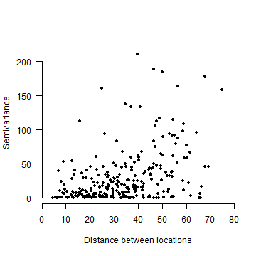
Plot a point cloud of spatial distance against the semivariance (Figure 10.13).
# semivariance
semivar <- dz^2 / 2
plot(dp, semivar, xlim=c(0, 80), ylim=c(0,220), xlab=c('Distance between locations'),
     ylab=c('Semivariance'), pch=20, axes=FALSE, xaxs="i")
axis(1, at=seq(0,80,10))
axis(2, las=1)
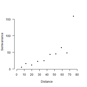
And plotting semivariance in bins
# choose a bin width (in spatial distance)
binwidth <- 8
# assign a lag (bin number) to each record
lag <- floor(dp/binwidth) + 1
# average value for each lag
lsv <- tapply(semivar, lag, mean)
# compute the average distance for each lag
dlag <- tapply(dp, lag, mean)
plot(dlag, lsv, pch=20, axes=FALSE, xlab='Distance', ylab='Semivariance', xlim=c(0,80))
axis(1, at=seq(0,80,10))
axis(2, las=1)
Now continue with the interpolation chapter of the “Spatial Data Analysis” book.