Map overlay
Introduction
This document shows some example R code to do “overlays” and associated spatial data manipulation to accompany Chapter 11 in O’Sullivan and Unwin (2010). You have already seen many of this type of data manipulation in previsous labs. And we have done perhaps more advanced things using regression type models (including LDA and RandomForest). This lab is very much a review of what you have already seen: basic spatial data operations in R. Below are some of the key packages for spatial data analysis that we have been using.
sp - Defines classes (data structures) for points, lines, polygons, rasters, and their attributes, and related funcitons for e.g, plotting. The main classes are SpatialPoints, SpatialLines, SpatialPolygons, SpatialGrid (all also with ‘DataFrame’ appended if the geometries have attributes)
raster - Defines alternative classes for raster data (RasterLayer, RasterStack, RasterBrick) that can be used for very large data sets. The package also provides many functions to manipulate raster data. It also extends to sp and rgeos packages for manipulating vector type data
rgdal - Read or write spatial data files (raster uses it behind the scenes).
rgeos - Geometry manipulation for vector data (e.g. intersection of polygons) and related matters.
spatstat - The main package for point pattern analysis (here used for a density function).
Get the data
You can get the data for this tutorial with the “rspatial” package that you can install with the line below.
if (!require("rspatial")) remotes::install_github('rspatial/rspatial')
Selection by attribute
By now, you are well aware that in R, polygons and their attributes can be represented by a ‘SpatialPolygonsDataFrame’ (a class defined in the sp package). Here we use a SpatialPolygonsDataFrame of California counties.
library(rspatial)
library(raster)
counties <- sp_data('counties.rds')
Selection by attribute of elements of a SpatialPolygonsDataFrame is
similar to selecting rows from a data.frame. For example, to select
Yolo county by its name:
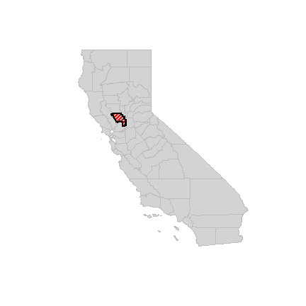
yolo <- counties[counties$NAME == 'Yolo', ]
plot(counties, col='light gray', border='gray')
plot(yolo, add=TRUE, density=20, lwd=2, col='red')
You can interactively select counties this way:
plot(counties)
s <- select(counties)
Intersection and buffer
I want to select the railroads in the city of Davis from the railroads in Yolo county. First read the data, and do an important sanity check: are the coordinate reference systems (“projections”) the same?
rail <- sp_data('yolo-rail.rds')
rail
## class       : SpatialLinesDataFrame
## features    : 4
## extent      : -122.0208, -121.5089, 38.31305, 38.9255  (xmin, xmax, ymin, ymax)
## crs         : +proj=longlat +datum=NAD83 +no_defs +ellps=GRS80 +towgs84=0,0,0
## variables   : 1
## names       :          FULLNAME
## min values  :      Abandoned RR
## max values  : Yolo Shortline RR
# removing attributes that I do not care about
rail <- geometry(rail)
class(rail)
## [1] "SpatialLines"
## attr(,"package")
## [1] "sp"
city <- sp_data('city.rds')
class(city)
## [1] "SpatialPolygonsDataFrame"
## attr(,"package")
## [1] "sp"
city <- geometry(city)
class(city)
## [1] "SpatialPolygons"
## attr(,"package")
## [1] "sp"
projection(yolo)
## [1] "+proj=longlat +datum=NAD83 +no_defs +ellps=GRS80 +towgs84=0,0,0"
projection(rail)
## [1] "+proj=longlat +datum=NAD83 +no_defs +ellps=GRS80 +towgs84=0,0,0"
projection(city)
## [1] "+proj=lcc +lat_1=38.33333333333334 +lat_2=39.83333333333334 +lat_0=37.66666666666666 +lon_0=-122 +x_0=2000000 +y_0=500000.0000000001 +datum=NAD83 +units=us-ft +no_defs +ellps=GRS80 +towgs84=0,0,0"
Ay, we are dealing with two different coordinate reference systems (projections)! Let’s settle for yet another one: Teale Albers (this is really the “Albers Equal Area projection with parameters suitable for California”. This particular set of parameters was used by an California State organization called the Teale Data Center, hence the name.
library(rgdal)
TA <- CRS("+proj=aea +lat_1=34 +lat_2=40.5 +lat_0=0 +lon_0=-120 +x_0=0 +y_0=-4000000 +datum=NAD83 +units=m +ellps=GRS80")
countiesTA <- spTransform(counties, TA)
## Warning in spTransform(xSP, CRSobj, ...): NULL source CRS comment, falling back
## to PROJ string
yoloTA <- spTransform(yolo, TA)
## Warning in spTransform(xSP, CRSobj, ...): NULL source CRS comment, falling back
## to PROJ string
railTA <- spTransform(rail, TA)
## Warning in spTransform(rail, TA): NULL source CRS comment, falling back to PROJ
## string
cityTA <- spTransform(city, TA)
## Warning in spTransform(city, TA): NULL source CRS comment, falling back to PROJ
## string
Another check, let’s see what county Davis is in, using two approaches. In the first one we get the centroid of Davis and do a point-in-polygon query.
dav <- coordinates(cityTA)
davis <- SpatialPoints(dav, proj4string=TA)
over(davis, countiesTA)
##   STATE COUNTY NAME LSAD LSAD_TRANS
## 0    06    113 Yolo   06     County
An alternative approach is to intersect the two polygon datasets.
i <- intersect(cityTA, countiesTA)
data.frame(i, area=area(i, byid=TRUE))
##   STATE COUNTY   NAME LSAD LSAD_TRANS       area
## 1    06    113   Yolo   06     County 25633905.4
## 2    06    095 Solano   06     County    78791.6
plot(cityTA, col='blue')
plot(yoloTA, add=TRUE, border='red', lwd=3)
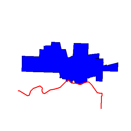
So we have a little sliver of Davis inside of Solano.
Everything looks OK. Now we can intersect rail and city, and make a buffer.
davis_rail <- intersect(railTA, cityTA)
Compute a 500 meter buffer around railroad inside Davis:
buf <- buffer(railTA, width=500)
rail_buf <- intersect(buf, cityTA)
plot(cityTA, col='light gray')
plot(rail_buf, add=TRUE, col='light blue', border='light blue')
plot(railTA, add=TRUE, lty=2, lwd=6)
plot(cityTA, add=TRUE)
plot(davis_rail, add=TRUE, col='red', lwd=6)
box()
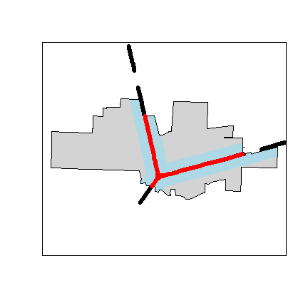
What is the percentage of the area of the city of Davis that is within 500 m of a railroad?
round(100 * area(rail_buf) / area(cityTA))
## [1] 31
Proximity
Which park in Davis is furthest, and which is closest to the railroad? First get the parks data.
parks <- sp_data('parks.rds')
proj4string(parks)
## [1] "+proj=lcc +lat_1=38.33333333333334 +lat_2=39.83333333333334 +lat_0=37.66666666666666 +lon_0=-122 +x_0=2000000 +y_0=500000.0000000001 +datum=NAD83 +units=us-ft +no_defs +ellps=GRS80 +towgs84=0,0,0"
parksTA <- spTransform(parks, TA)
## Warning in spTransform(xSP, CRSobj, ...): NULL source CRS comment, falling back
## to PROJ string
Now plot the parks that are the furthest and the nearest from a railroad.
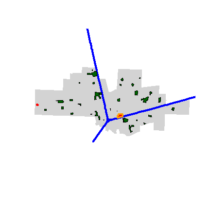
plot(cityTA, col='light gray', border='light gray')
plot(railTA, add=T, col='blue', lwd=4)
plot(parksTA, col='dark green', add=TRUE)
library(rgeos)
## rgeos version: 0.5-9, (SVN revision 684)
##  GEOS runtime version: 3.9.1-CAPI-1.14.2
##  Please note that rgeos will be retired by the end of 2023,
## plan transition to sf functions using GEOS at your earliest convenience.
##  GEOS using OverlayNG
##  Linking to sp version: 1.4-6
##  Polygon checking: TRUE
d <- gDistance(parksTA, railTA, byid=TRUE)
dmin <- apply(d, 2, min)
parksTA$railDist <- dmin
i <- which.max(dmin)
data.frame(parksTA)[i,]
##              PARK     PARKTYPE            ADDRESS railDist
## 25 Whaleback Park NEIGHBORHOOD 1011 MARINA CIRCLE 4330.938
plot(parksTA[i, ], add=TRUE, col='red', lwd=3, border='red')
j <- which.min(dmin)
data.frame(parksTA)[j,]
##                    PARK     PARKTYPE         ADDRESS railDist
## 13 Toad Hollow Dog Park NEIGHBORHOOD 1919 2ND STREET 23.83512
plot(parksTA[j, ], add=TRUE, col='red', lwd=3, border='orange')
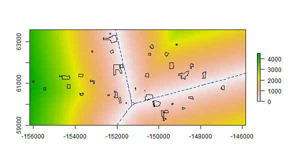
Another way to approach this is to first create a raster with distance to the railroad values. Here we compute the average distance to any place inside the park, not to its border. You could also compute the distance to the centroid of a park.
library(raster)
# use cityTA to set the geogaphic extent
r <- raster(cityTA)
# arbitrary resolution
dim(r) <- c(50, 100)
# rasterize the railroad lines
r <- rasterize(railTA, r, field=1)
# compute distance
d <- distance(r)
# extract distance values for polygons
dp <- extract(d, parksTA, fun=mean, small=TRUE)
dp <- data.frame(parksTA$PARK, dist=dp)
dp <- dp[order(dp$dist), ]
plot(d)
plot(parksTA, add=TRUE)
plot(railTA, add=T, col='blue', lty=2)
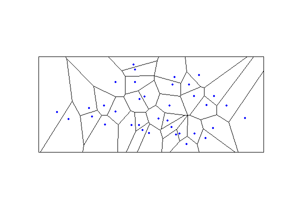
Thiessen polygons
Here I compute Thiessen (or Voronoi) polygons for the Davis parks. Each polygon shows the area that is closest to (the centroid of) a particular park.
library(dismo)
centroids <- coordinates(parksTA)
v <- voronoi(centroids)
plot(v)
points(centroids, col='blue', pch=20)
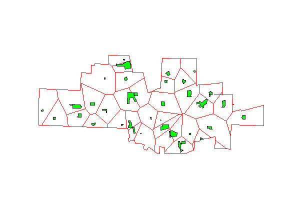
To keep the polygons within Davis.
proj4string(v) <- TA
vc <- intersect(v, cityTA)
plot(vc, border='red')
plot(parksTA, add=T, col='green')
Fields
Raster data
raster data can be read with readGDAL to get a SpatialGridDataFrame. But I prefer to use the raster package to create Raster* objects. Raster* stands for RasterLayer, RasterStack, or RasterBrick. See the vignette for the raster package for more details: http://cran.r-project.org/web/packages/raster/vignettes/Raster.pdf
library(raster)
# get a RasterLayer with elevation data
alt <- sp_data("elevation")
alt
## class      : RasterLayer
## dimensions : 239, 474, 113286  (nrow, ncol, ncell)
## resolution : 0.008333333, 0.008333333  (x, y)
## extent     : -123.95, -120, 37.3, 39.29167  (xmin, xmax, ymin, ymax)
## crs        : +proj=longlat +datum=WGS84 +no_defs +ellps=WGS84 +towgs84=0,0,0
## source     : memory
## names      : elevation
## values     : -30, 2963  (min, max)
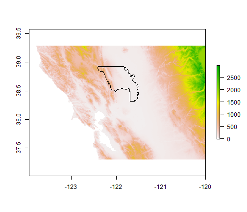
The CRS of RasterLayer ‘alt’ is “lon/lat””, and so is the CRS of ‘yolo’. However, ‘yolo’ has a different datum (NAD83) than ‘alt’ (WGS84). While there is no real difference between these, this will lead to errors, so we first transform yolo. It is generally better to match vector data to raster data than vice versa.
yolo <- spTransform(yolo, crs(alt))
## Warning in spTransform(xSP, CRSobj, ...): NULL source CRS comment, falling back
## to PROJ string
## Warning in spTransform(xSP, CRSobj, ...): NULL target CRS comment, falling back
## to PROJ string
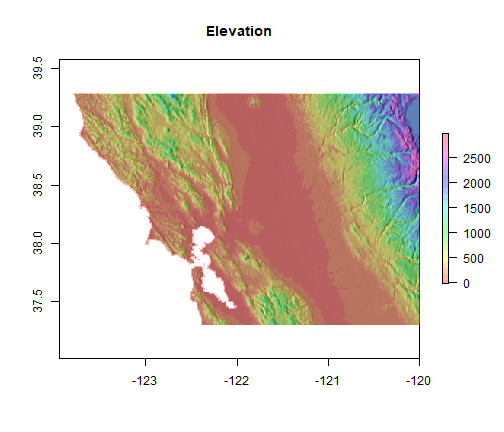
plot(alt)
plot(yolo, add=TRUE)
Shaded relief is always nice to look at.
slope <- terrain(alt, opt='slope')
aspect <- terrain(alt, opt='aspect')
hill <- hillShade(slope, aspect, 40, 270)
plot(hill, col=grey(0:100/100), legend=FALSE, main='Elevation')
plot(alt, col=rainbow(25, alpha=0.35), add=TRUE)
You can also try the plot3D function in the rasterVis package.
Query
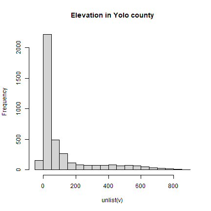
Now extract elevation data for Yolo county.
v <- extract(alt, yolo)
hist(unlist(v), main='Elevation in Yolo county')
Another approach:
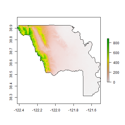
# cut out a rectangle (extent) of Yolo
yalt <- crop(alt, yolo)
# 'mask' out the values outside Yolo
ymask <- mask(yalt, yolo)
# summary of the raster cell values
summary(ymask)
##         elevation
## Min.           -1
## 1st Qu.         6
## Median         30
## 3rd Qu.       110
## Max.          882
## NA's         4171
plot(ymask)
plot(yolo, add=T)
You can also get values (query) by clicking on the map (use
click(alt))
Exercise
We want to travel by train in Yolo county and we want to get as close as possible to a hilly area; whenever we get there we’ll jump from the train. It turns out that the railroad tracks are not all connected, we will ignore that inconvenience.
Define “hilly” as some vague notion of a combination of high elevation and slope (in degrees). Use some of the functions you have seen above, as well as function ‘distance’ to create a plot of distance from the railroad against hillyness. Make a map to illustrate the result, showing where you get off the train, where you go to, and what the elevation and slope profile would be if you follow the shortest (as the crow flies) path.
Bonus: use package gdistance to find the least-cost path between
these two points (assign a cost to slope, perhaps using Tobler’s hiking
function).