Spatial autocorrelation
Introduction
This handout accompanies Chapter 7 in O’Sullivan and Unwin (2010).
First load the rspatial package, to get access to the data we will
use.
if (!require("rspatial")) remotes::install_github('rspatial/rspatial')
library(rspatial)
The area of a polygon
Create a polygon like in Figure 7.2 (page 192).
pol <- matrix(c(1.7, 2.6, 5.6, 8.1, 7.2, 3.3, 1.7, 4.9, 7, 7.6, 6.1, 2.7, 2.7, 4.9), ncol=2)
library(raster)
sppol <- spPolygons(pol)
For illustration purposes, we create the “negative area” polygon as well
negpol <- rbind(pol[c(1,6:4),], cbind(pol[4,1], 0), cbind(pol[1,1], 0))
spneg <- spPolygons(negpol)
Now plot
cols <- c('light gray', 'light blue')
plot(sppol, xlim=c(1,9), ylim=c(1,10), col=cols[1], axes=FALSE, xlab='', ylab='',
      lwd=2, yaxs="i", xaxs="i")
plot(spneg, col=cols[2], add=T)
plot(spneg, add=T, density=8, angle=-45, lwd=1)
segments(pol[,1], pol[,2], pol[,1], 0)
text(pol, LETTERS[1:6], pos=3, col='red', font=4)
arrows(1, 1, 9, 1, 0.1, xpd=T)
arrows(1, 1, 1, 9, 0.1, xpd=T)
text(1, 9.5, 'y axis', xpd=T)
text(10, 1, 'x axis', xpd=T)
legend(6, 9.5, c('"positive" area', '"negative" area'), fill=cols, bty = "n")
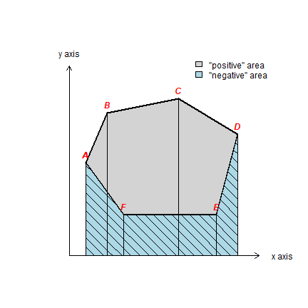
Compute area
p <- rbind(pol, pol[1,])
x <- p[-1,1] - p[-nrow(p),1]
y <- (p[-1,2] + p[-nrow(p),2]) / 2
sum(x * y)
## [1] 23.81
Or simply use an existing function
# make sure that the coordinates are interpreted as planar (not longitude/latitude)
crs(sppol) <- '+proj=utm +zone=1'
area(sppol)
## [1] 23.81
Contact numbers
“Contact numbers” for the lower 48 states. Get the polygons:
library(raster)
usa <- raster::getData('GADM', country='USA', level=1)
usa <- usa[! usa$NAME_1 %in% c('Alaska', 'Hawaii'), ]
To find adjacent polygons, we can use the spdep package.
library(spdep)
We use poly2nb to create a neighbors-list. And from that a neighbors
matrix.
# patience, this takes a while:
wus <- poly2nb(usa, row.names=usa$OBJECTID, queen=FALSE)
wus
## Neighbour list object:
## Number of regions: 49
## Number of nonzero links: 220
## Percentage nonzero weights: 9.162849
## Average number of links: 4.489796
wmus <- nb2mat(wus, style='B', zero.policy = TRUE)
dim(wmus)
## [1] 49 49
Compute the number of neighbors for each state.
i <- rowSums(wmus)
round(100 * table(i) / length(i), 1)
## i
##    1    2    3    4    5    6    7    8
##  2.0 10.2 16.3 22.4 16.3 26.5  2.0  4.1
Apparently, I am using a different data set than OSU (compare the above
with table 7.1). By changing the level argument to 2 in the
getData function you can run the same for counties. Which county has
13 neighbors?
Spatial structure
Read the Auckland data.
if (!require("rspatial")) remotes::install_github('rspatial/rspatial')
library(rspatial)
pols <- sp_data("auctb.rds")
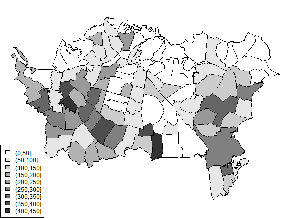
I did not have the tuberculosis data so I guesstimated them from figure 7.7. Compare:
par(mai=c(0,0,0,0))
classes <- seq(0,450,50)
cuts <- cut(pols$TB, classes)
n <- length(classes)
cols <- rev(gray(0:n / n))
plot(pols, col=cols[as.integer(cuts)])
legend('bottomleft', levels(cuts), fill=cols)
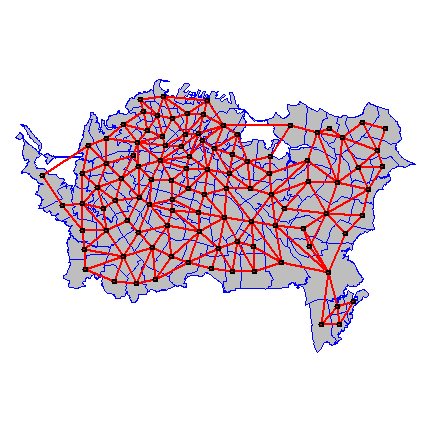
Create a Rooks’ case neighborhood object.
wr <- poly2nb(pols, row.names=pols$Id, queen=FALSE)
class(wr)
## [1] "nb"
summary(wr)
## Neighbour list object:
## Number of regions: 103
## Number of nonzero links: 504
## Percentage nonzero weights: 4.750683
## Average number of links: 4.893204
## Link number distribution:
##
##  2  3  4  5  6  7  8
##  4 14 21 30 22  8  4
## 4 least connected regions:
## 5 29 46 82 with 2 links
## 4 most connected regions:
## 3 4 36 83 with 8 links
Plot the links between the polygons.
par(mai=c(0,0,0,0))
plot(pols, col='gray', border='blue')
xy <- coordinates(pols)
plot(wr, xy, col='red', lwd=2, add=TRUE)
We can create a matrix from the links list.
wm <- nb2mat(wr, style='B')
dim(wm)
## [1] 103 103
And inspect the content or wr and wm
wr[1:6]
## [[1]]
## [1] 28 53 73 74 75 76 77
##
## [[2]]
## [1] 30 73 74
##
## [[3]]
## [1] 33 35 44 53
##
## [[4]]
## [1] 28 29 31 41 43 75 76 97
##
## [[5]]
## [1] 32 37 39 64 78 79 81 86
##
## [[6]]
## [1]  7 11
wm[1:6,1:11]
##   [,1] [,2] [,3] [,4] [,5] [,6] [,7] [,8] [,9] [,10] [,11]
## 0    0    0    0    0    0    0    0    0    0     0     0
## 1    0    0    0    0    0    0    0    0    0     0     0
## 2    0    0    0    0    0    0    0    0    0     0     0
## 3    0    0    0    0    0    0    0    0    0     0     0
## 4    0    0    0    0    0    0    0    0    0     0     0
## 5    0    0    0    0    0    0    1    0    0     0     1
Question 1:Explain the meaning of the first lines returned by wr[1:6])
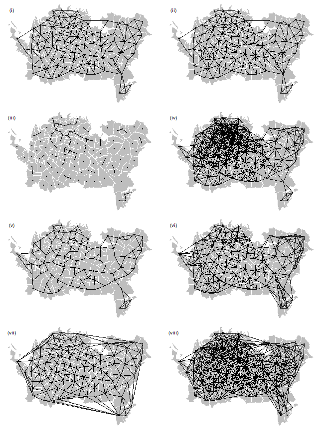
Now let’s recreate Figure 7.6 (page 202).
We already have the first one (Rook’s case adjacency, plotted above). Queen’s case adjacency:
wq <- poly2nb(pols, row.names=pols$Id, queen=TRUE)
Distance based:
wd1 <- dnearneigh(xy, 0, 1000)
wd25 <- dnearneigh(xy, 0, 2500)
Nearest neighbors:
k3 <- knn2nb(knearneigh(xy, k=3))
k6 <- knn2nb(knearneigh(xy, k=6))
Delauny:
library(deldir)
d <- deldir(xy[,1], xy[,2], suppressMsge=TRUE)
Lag-two Rook:
wr2 <- wr
for (i in 1:length(wr)) {
    lag1 <- wr[[i]]
    lag2 <- wr[lag1]
    lag2 <- sort(unique(unlist(lag2)))
    lag2 <- lag2[!(lag2 %in% c(wr[[i]], i))]
    wr2[[i]] <- lag2
}
And now we plot them all using the plotit function.
  plotit <- function(nb, lab='') {
  plot(pols, col='gray', border='white')
  plot(nb, xy, add=TRUE, pch=20)
  text(2659066, 6482808, paste0('(', lab, ')'), cex=1.25)
}
par(mfrow=c(4, 2), mai=c(0,0,0,0))
plotit(wr, 'i')
plotit(wq, 'ii')
plotit(wd1, 'iii')
plotit(wd25, 'iv')
plotit(k3, 'v')
plotit(k6, 'vi')
plot(pols, col='gray', border='white')
plot(d, wlines='triang', add=TRUE, pch=20)
text(2659066, 6482808, '(vii)', cex=1.25)
plotit(wr2, 'viii')
Moran’s I
Below I compute Moran’s index according to formula 7.7 on page 205 of OSU.
The number of observations
n <- length(pols)
Values ‘y’ and ‘ybar’ (the mean of y).
y <- pols$TB
ybar <- mean(y)
Now we need
That is, (yi-ybar)(yj-ybar) for all pairs. I show two methods to compute that.
Method 1:
dy <- y - ybar
g <- expand.grid(dy, dy)
yiyj <- g[,1] * g[,2]
Method 2:
yi <- rep(dy, each=n)
yj <- rep(dy, n)
yiyj <- yi * yj
Make a matrix of the multiplied pairs
pm <- matrix(yiyj, ncol=n)
round(pm[1:6, 1:9])
##        [,1]  [,2]   [,3]   [,4]  [,5]   [,6]   [,7]   [,8]  [,9]
## [1,]  22778  4214 -12538  30776 -3181 -10727 -17821 -12387 -5445
## [2,]   4214   780  -2320   5694  -589  -1985  -3297  -2292 -1007
## [3,] -12538 -2320   6902 -16941  1751   5905   9810   6819  2997
## [4,]  30776  5694 -16941  41584 -4298 -14494 -24079 -16737 -7357
## [5,]  -3181  -589   1751  -4298   444   1498   2489   1730   760
## [6,] -10727 -1985   5905 -14494  1498   5052   8393   5834  2564
And multiply this matrix with the weights to set to zero the value for the pairs that are not adjacent.
pmw <- pm * wm
wm[1:6, 1:9]
##   [,1] [,2] [,3] [,4] [,5] [,6] [,7] [,8] [,9]
## 0    0    0    0    0    0    0    0    0    0
## 1    0    0    0    0    0    0    0    0    0
## 2    0    0    0    0    0    0    0    0    0
## 3    0    0    0    0    0    0    0    0    0
## 4    0    0    0    0    0    0    0    0    0
## 5    0    0    0    0    0    0    1    0    0
round(pmw[1:6, 1:9])
##   [,1] [,2] [,3] [,4] [,5] [,6] [,7] [,8] [,9]
## 0    0    0    0    0    0    0    0    0    0
## 1    0    0    0    0    0    0    0    0    0
## 2    0    0    0    0    0    0    0    0    0
## 3    0    0    0    0    0    0    0    0    0
## 4    0    0    0    0    0    0    0    0    0
## 5    0    0    0    0    0    0 8393    0    0
We sum the values, to get this bit of Moran’s I:
spmw <- sum(pmw)
spmw
## [1] 1523422
The next step is to divide this value by the sum of weights. That is easy.
smw <- sum(wm)
sw  <- spmw / smw
And compute the inverse variance of y
vr <- n / sum(dy^2)
The final step to compute Moran’s I
MI <- vr * sw
MI
## [1] 0.2643226
This is how you can (theoretically) estimate the expected value of Moran’s I. That is, the value you would get in the absence of spatial autocorrelation. Note that it is not zero for small values of n.
EI <- -1/(n-1)
EI
## [1] -0.009803922
After doing this ‘by hand’, now let’s use the spdep package to compute
Moran’s I and do a significance test. To do this we need to create a
listw type spatial weights object. To get the same value as above we
use style='B' to use binary (TRUE/FALSE) distance weights.
ww <- nb2listw(wr, style='B')
ww
## Characteristics of weights list object:
## Neighbour list object:
## Number of regions: 103
## Number of nonzero links: 504
## Percentage nonzero weights: 4.750683
## Average number of links: 4.893204
##
## Weights style: B
## Weights constants summary:
##     n    nn  S0   S1    S2
## B 103 10609 504 1008 10672
On to the moran function. Have a look at ?moran. The function is
defined as moran(y, ww, n, Szero(ww)). Note the odd arguments n
and S0. I think they are odd, because ww has that information.
Anyway, we supply them and it works. There probably are cases where it
makes sense to use other values.
moran(pols$TB, ww, n=length(ww$neighbours), S0=Szero(ww))
## $I
## [1] 0.2643226
##
## $K
## [1] 3.517442
Note that the global sum ow weights
Szero(ww)
## [1] 504
Should be the same as
sum(pmw != 0)
## [1] 504
Now we can test for significance. First analytically, using linear regression based logic and assumptions.
moran.test(pols$TB, ww, randomisation=FALSE)
##
##  Moran I test under normality
##
## data:  pols$TB
## weights: ww
##
## Moran I statistic standard deviate = 4.478, p-value = 3.767e-06
## alternative hypothesis: greater
## sample estimates:
## Moran I statistic       Expectation          Variance
##       0.264322626      -0.009803922       0.003747384
And now using Monte Carlo simulation — which is the preferred method. In fact, the only good method to use.
moran.mc(pols$TB, ww, nsim=99)
##
##  Monte-Carlo simulation of Moran I
##
## data:  pols$TB
## weights: ww
## number of simulations + 1: 100
##
## statistic = 0.26432, observed rank = 100, p-value = 0.01
## alternative hypothesis: greater
Question 2: How do you interpret these results (the significance tests)?
Question 3: What would a good value be for ``nsim``?
To make a Moran scatter plot we first get the neighbouring values for each value.
n <- length(pols)
ms <- cbind(id=rep(1:n, each=n), y=rep(y, each=n), value=as.vector(wm * y))
Remove the zeros
ms <- ms[ms[,3] > 0, ]
And compute the average neighbour value
ams <- aggregate(ms[,2:3], list(ms[,1]), FUN=mean)
ams <- ams[,-1]
colnames(ams) <- c('y', 'spatially lagged y')
head(ams)
##     y spatially lagged y
## 1 271           135.1429
## 2 148           154.3333
## 3  37           142.2500
## 4 324           142.6250
## 5  99            71.6250
## 6  49            14.5000
Finally, the plot.
plot(ams)
reg <- lm(ams[,2] ~ ams[,1])
abline(reg, lwd=2)
abline(h=mean(ams[,2]), lt=2)
abline(v=ybar, lt=2)
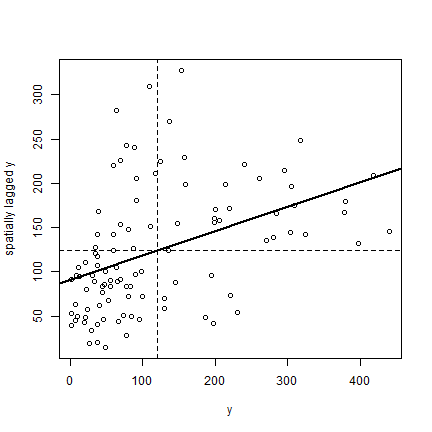
Note that the slope of the regression line:
coefficients(reg)[2]
##  ams[, 1]
## 0.2746281
is almost the same as Moran’s I.
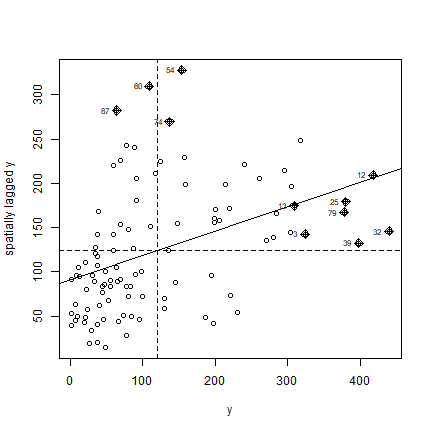
Here is a more direct approach to accomplish the same thing (but hopefully the above makes it clearer how this is actually computed). Note the row standardisation of the weights matrix:
rwm <- mat2listw(wm, style='W')
# Checking if rows add up to 1
mat <- listw2mat(rwm)
apply(mat, 1, sum)[1:15]
##  0  1  2  3  4  5  6  7  8  9 10 11 12 13 14
##  1  1  1  1  1  1  1  1  1  1  1  1  1  1  1
Now we can plot
moran.plot(y, rwm)
Question 4: Show how to use the ‘geary’ function to compute Geary’s C
Question 5: Write your own Monte Carlo simulation test to compute p-values for Moran’sI, replicating the results we obtained with the function from spdep. Show a figure similar to Figure 7.9 in OSU.
Question 6: Write your own Geary C function, by completing the function below
gearyC <- ((n-1)/sum(( "----")\^2)) * sum(wm * (" --- ")\^2) / (2 * sum(wm))