Spatial prediction
This chapters shows some examples for making spatial prediction with
different types of models. Using the predict and interpolate
methods.
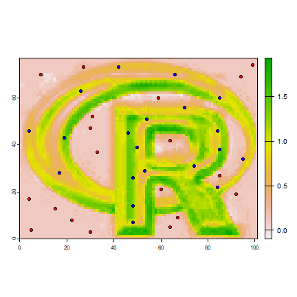
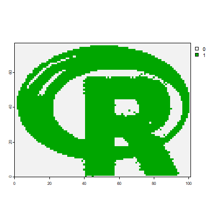
The is the data we use.
library(terra)
logo <- rast(system.file("ex/logo.tif", package="terra"))
names(logo) <- c("red", "green", "blue")
p <- matrix(c(48, 48, 48, 53, 50, 46, 54, 70, 84, 85, 74, 84, 95, 85,
   66, 42, 26, 4, 19, 17, 7, 14, 26, 29, 39, 45, 51, 56, 46, 38, 31,
   22, 34, 60, 70, 73, 63, 46, 43, 28), ncol=2)
a <- matrix(c(22, 33, 64, 85, 92, 94, 59, 27, 30, 64, 60, 33, 31, 9,
   99, 67, 15, 5, 4, 30, 8, 37, 42, 27, 19, 69, 60, 73, 3, 5, 21,
   37, 52, 70, 74, 9, 13, 4, 17, 47), ncol=2)
xy <- rbind(cbind(1, p), cbind(0, a))
# extract predictor values for points
e <- extract(logo, xy[,2:3])
# combine with response
v <- data.frame(cbind(pa=xy[,1], e))
Predict
GLM
A general linear model (GLM)
#build a model, here with glm
model <- glm(formula=pa~., data=v)
#predict to a raster
r1 <- predict(logo, model)
plot(r1)
points(p, bg='blue', pch=21)
points(a, bg='red', pch=21)
# logistic regression
model <- glm(formula=pa~., data=v, family="binomial")
## Warning: glm.fit: algorithm did not converge
## Warning: glm.fit: fitted probabilities numerically 0 or 1 occurred
r1log <- predict(logo, model, type="response")
# use a modified function to get the probability and standard error
# from the glm model. The values returned by "predict" are in a list,
# and this list needs to be transformed to a matrix
predfun <- function(model, data) {
  v <- predict(model, data, se.fit=TRUE)
  cbind(p=as.vector(v$fit), se=as.vector(v$se.fit))
}
r2 <- predict(logo, model, fun=predfun)
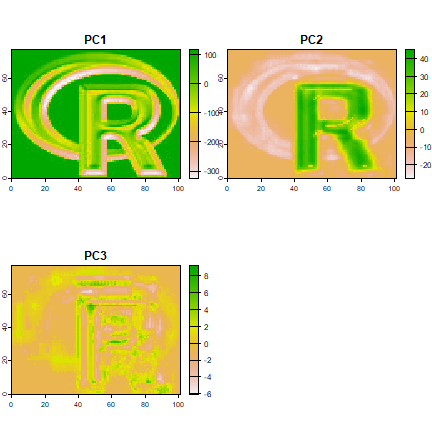
Principal components
Here using sampling to simulate an object too large to feed all its values to prcomp
sr <- values(spatSample(logo, 100, as.raster=TRUE))
pca <- prcomp(sr)
x <- predict(logo, pca)
plot(x)
library(pls)
##
## Attaching package: 'pls'
## The following object is masked from 'package:stats':
##
##     loadings
model <- plsr(formula=pa~., data=v)
# this returns an array:
predict(model, v[1:5,])
## , , 1 comps
##
##          pa
## 1 0.4918092
## 2 0.7463392
## 3 0.7774598
## 4 0.3499635
## 5 0.6490389
##
## , , 2 comps
##
##          pa
## 1 0.6875604
## 2 1.0224901
## 3 1.0499689
## 4 0.5055191
## 5 0.9808813
##
## , , 3 comps
##
##          pa
## 1 0.8172886
## 2 1.1435330
## 3 1.1717481
## 4 0.4949081
## 5 0.8458842
# write a function to turn that into a matrix
pfun <- function(x, data) {
   y <- predict(x, data)
   d <- dim(y)
   dim(y) <- c(prod(d[1:2]), d[3])
   y
}
pp <- predict(logo, model, fun=pfun)
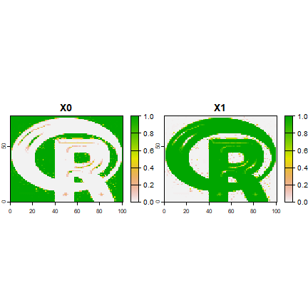
Random Forest
library(randomForest)
## randomForest 4.7-1.2
## Type rfNews() to see new features/changes/bug fixes.
rfmod <- randomForest(pa ~., data=v)
## Warning in randomForest.default(m, y, ...): The response has five or fewer
## unique values.  Are you sure you want to do regression?
## note the additional argument "type='response'" that is
## passed to predict.randomForest
r3 <- predict(logo, rfmod, type='response')
## get class membership probabilities
vv <- v
vv$pa <- as.factor(vv$pa)
rfmod2 <- randomForest(pa ~., data=vv)
r4 <- predict(logo, rfmod2, type='prob')
plot(r4, range=c(0,1))
cforest
cforest is an alternative Random Forest implementation. Here an example
with a factors argument
library(party)
## Loading required package: grid
##
## Attaching package: 'grid'
## The following object is masked from 'package:terra':
##
##     depth
## Loading required package: mvtnorm
## Loading required package: modeltools
## Loading required package: stats4
## Loading required package: strucchange
## Loading required package: zoo
##
## Attaching package: 'zoo'
## The following object is masked from 'package:terra':
##
##     time<-
## The following objects are masked from 'package:base':
##
##     as.Date, as.Date.numeric
## Loading required package: sandwich
m <- cforest(pa~., control=cforest_unbiased(mtry=3), data=v)
# the second argument in party:::predict.RandomForest
# is "OOB", and not "newdata" or similar. We need to write a wrapper
# predict function to deal with this
predfun <- function(m, d, ...) predict(m, newdata=d, ...)
pc <- predict(logo, m, OOB=TRUE, fun=predfun)
With a knn model, we can use “app” instead of “predict”
library(class)
cl <- factor(c(rep(1, nrow(p)), rep(0, nrow(a))))
train <- extract(logo, rbind(p, a))
k <- app(logo, function(x) as.integer(as.character(knn(train, x, cl))))
plot(k)
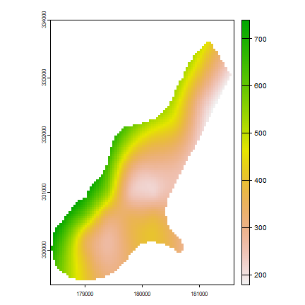
Interpolate
Thin plate spline interpolation with x and y only
library(terra)
# example data
r <-rast(system.file("ex/meuse.tif", package="terra"))
ra <- aggregate(r, 10)
xy <- data.frame(xyFromCell(ra, 1:ncell(ra)))
v <- values(ra)
# Thin plate spline model
library(fields)
tps <- Tps(xy, v)
## Warning:
## Grid searches over lambda (nugget and sill variances) with  minima at the endpoints:
##   (GCV) Generalized Cross-Validation
##    minimum at  right endpoint  lambda  =  6.369487e-05 (eff. df= 17.10001 )
x <- rast(r)
# use model to predict values at all locations
p <- interpolate(x, tps)
p <- mask(p, r)
plot(p)
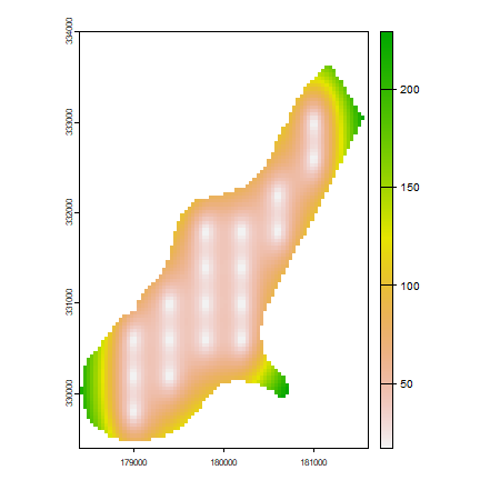
# change the fun from predict to fields::predictSE to get the TPS standard error
se <- interpolate(x, tps, fun=predictSE)
se <- mask(se, r)
plot(se)
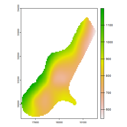
Add another predictor variable; let”s call it elevation
elevation <- (init(r, "x") * init(r, "y")) / 100000000
names(elevation) <- "elev"
elevation <- mask(elevation, r)
z <- extract(elevation, vect(xy, c("x", "y")), fun=function(x)x[1])
z <- z[,2,drop=FALSE]
# add as another independent variable
vv <- na.omit(cbind(xy, z, v))
tps2 <- Tps(vv[,1:3], vv[,4])
## Warning:
## Grid searches over lambda (nugget and sill variances) with  minima at the endpoints:
##   (GCV) Generalized Cross-Validation
##    minimum at  right endpoint  lambda  =  0.0003764795 (eff. df= 17.10001 )
#p2 <- interpolate(elevation, tps2)
#plot(p2)
# as a linear coveriate
tps3 <- Tps(vv[,1:2], vv[,4], Z=vv[,3])
## Warning:
## Grid searches over lambda (nugget and sill variances) with  minima at the endpoints:
##   (GCV) Generalized Cross-Validation
##    minimum at  right endpoint  lambda  =  6.464444e-05 (eff. df= 17.10047 )
# Z is a separate argument in Krig.predict, so we need a new function
# Internally (in interpolate) a matrix is formed of x, y, and elev (Z)
pfun <- function(model, x, ...) {
   predict(model, x[,1:2], Z=x[,3], ...)
}
p3 <- interpolate(elevation, tps3, fun=pfun)
plot(p3)
inverse distance weighted (IDW)
library(gstat)
data(meuse, package="sp")
r <- rast(system.file("ex/meuse.tif", package="terra"))
mg <- gstat(id = "zinc", formula = zinc~1, locations = ~x+y, data=meuse,
            nmax=7, set=list(idp = .5))
z <- interpolate(r, mg, debug.level=0)
Kriging
Kriging with gstat examples. Examples provided by Maurizio Marchi
orinary kriging
v <- variogram(log(zinc)~1, ~x+y, data=meuse)
mv <- fit.variogram(v, vgm(1, "Sph", 300, 1))
gOK <- gstat(NULL, "log.zinc", log(zinc)~1, meuse, locations=~x+y, model=mv)
OK <- interpolate(r, gOK, debug.level=0)
plot(OK)
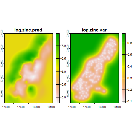
universial kriging
vu <- variogram(log(zinc)~elev, ~x+y, data=meuse)
mu <- fit.variogram(vu, vgm(1, "Sph", 300, 1))
gUK <- gstat(NULL, "log.zinc", log(zinc)~elev, meuse, locations=~x+y, model=mu)
names(r) <- "elev"
UK <- interpolate(r, gUK, debug.level=0)
plot(UK)
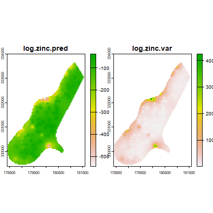
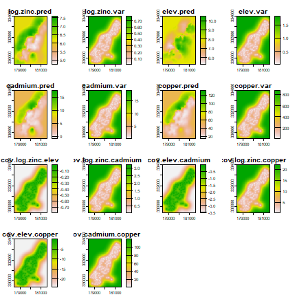
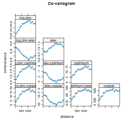
co-kriging
gCoK <- gstat(NULL, 'log.zinc', log(zinc)~1, meuse, locations=~x+y)
gCoK <- gstat(gCoK, 'elev', elev~1, meuse, locations=~x+y)
gCoK <- gstat(gCoK, 'cadmium', cadmium~1, meuse, locations=~x+y)
gCoK <- gstat(gCoK, 'copper', copper~1, meuse, locations=~x+y)
coV <- variogram(gCoK)
plot(coV, type='b', main='Co-variogram')
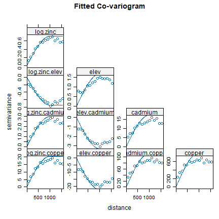
coV.fit <- fit.lmc(coV, gCoK, vgm(model='Sph', range=1000))
coV.fit
## data:
## log.zinc : formula = log(zinc)`~`1 ; data dim = 155 x 12
## elev : formula = elev`~`1 ; data dim = 155 x 12
## cadmium : formula = cadmium`~`1 ; data dim = 155 x 12
## copper : formula = copper`~`1 ; data dim = 155 x 12
## variograms:
##                  model       psill range
## log.zinc           Sph   0.7132435  1000
## elev               Sph   1.6908552  1000
## cadmium            Sph  17.4957356  1000
## copper             Sph 809.4027563  1000
## log.zinc.elev      Sph  -0.7404289  1000
## log.zinc.cadmium   Sph   2.9802854  1000
## elev.cadmium       Sph  -3.2983554  1000
## log.zinc.copper    Sph  20.4199742  1000
## elev.copper        Sph -22.4955673  1000
## cadmium.copper     Sph 111.1393673  1000
## ~x + y
## <environment: 0x00000235e5425ea8>
plot(coV, coV.fit, main='Fitted Co-variogram')
coK <- interpolate(r, coV.fit, debug.level=0)
plot(coK)