High-level methods
Several ‘high level’ methods (functions) have been implemented for
SpatRaster objects. ‘High level’ refers to methods that you would
normally find in a GIS program that supports raster data. Here we
briefly discuss some of these. See the help files for more detailed
descriptions.
The high-level methods have some arguments in common. The first argument
is typically ‘x’ or ‘object’ and in most cases it is a SpatRaster or
a SpatVector. It is followed by one or more arguments specific to
the method (either additional SpatRaster objects or other
arguments), followed by a filename=“” and “…” arguments.
The default filename is an empty character ““. If you do not specify a
filename, the default action for the method is to return a terra
object that only exists in memory. However, if the method deems that the
terra object to be created would be too large to hold memory it is
written to a temporary file instead.
The “…” argument allows for setting additional arguments that are relevant when writing values to a file: the file format, datatype (e.g. integer or real values), and a to indicate whether existing files should be overwritten.
Modifying a SpatRaster object
There are several methods that deal with modifying the spatial extent of
SpatRaster objects. The crop method lets you take a geographic
subset of a larger terra object. You can crop a SpatRaster by
providing an extent object or another spatial object from which an
extent can be extracted (objects from classes deriving from Raster and
from Spatial in the sp package). An easy way to get an extent object is
to plot a SpatRaster and then use drawExtent to visually
determine the new extent (bounding box) to provide to the crop method.
trim crops a SpatRaster by removing the outer rows and columns
that only contain NA values. In contrast, extend adds new rows
and/or columns with NA values. The purpose of this could be to
create a new SpatRaster with the same Extent of another larger
SpatRaster such that the can be used together in other methods.
The merge method lets you merge 2 or more SpatRaster objects
into a single new object. The input objects must have the same
resolution and origin (such that their cells neatly fit into a single
larger raster). If this is not the case you can first adjust one of the
SpatRaster objects with use (dis)aggregate or resample.
aggregate and disagg allow for changing the resolution (cell
size) of a SpatRaster object. In the case of aggregate, you need
to specify a function determining what to do with the grouped cell
values (e.g. mean). It is possible to specify different
(dis)aggregation factors in the x and y direction. aggregate and
disagg are the best methods when adjusting cells size only, with an
integer step (e.g. each side 2 times smaller or larger), but in some
cases that is not possible.
For example, you may need nearly the same cell size, while shifting the
cell centers. In those cases, the resample method can be used. It
can do either nearest neighbor assignments (for categorical data) or
bilinear interpolation (for numerical data). Simple linear shifts of a
Raster object can be accomplished with the shift method or with the
extent method. resample should not be used to create a
SpatRaster object with much larger resolution. If such adjustments need
to be made then you can first use aggregate.
With the warp method you can transform values of a SpatRaster to
a new object with a different coordinate reference system.
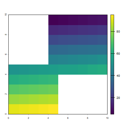
Here are some simple examples.
library(terra)
## terra 1.9.21
r <- rast(ncol=10, nrow=10, xmin=0, xmax=10, ymin=0, ymax=10)
values(r) <- 1:ncell(r)
ra <- aggregate(r, 2)
r1 <- crop(r, ext(0, 5, 0, 5))
r2 <- crop(r, ext(4, 10, 4, 10))
m <- merge(r1, r2, filename='test.tif', overwrite=TRUE)
plot(m)
bf lets you flip the data (reverse order) in horizontal or vertical
direction – typically to correct for a ‘communication problem’ between
different R packages or a misinterpreted file. rotate lets you
rotate longitude/latitude rasters that have longitudes from 0 to 360
degrees (often used by climatologists) to the standard -180 to 180
degrees system. With t you can rotate a SpatRaster object 90
degrees.
lapp
The lapp (for layer-apply) method can be used as an alternative to
the raster algebra discussed above. Like the methods discussed in the
following subsections provide either easy to use short-hand, or more
efficient computation for large (file based) objects.
With lapp you can combine multiple SpatRaster objects. The related
method mask removes all values from one layer that are NA in
another layer, and cover combines two layers by taking the values of
the first layer except where these are NA.
app
The app method allows you to do a computation across the layers of a
terra object by providing a function (like apply on a matrix or
data.frame). If you supply a SpatRaster, another SpatRaster is
returned. tapp computes summary type layers for subsets of a
SpatRaster (like tapply on a matrix or data.frame).
classify
You can use cut or classify to replace ranges of values with
single values, or subs to substitute (replace) single values with
other values.
r <- rast(ncol=3, nrow=2)
values(r) <- 1:ncell(r)
values(r)
##      lyr.1
## [1,]     1
## [2,]     2
## [3,]     3
## [4,]     4
## [5,]     5
## [6,]     6
s <- app(r, fun=function(x){ x[x < 4] <- NA; return(x)} )
as.matrix(s)
##      lyr.1
## [1,]    NA
## [2,]    NA
## [3,]    NA
## [4,]     4
## [5,]     5
## [6,]     6
t <- lapp(c(r, s), fun=function(x, y){ x / (2 * sqrt(y)) + 5 } )
as.matrix(t)
##          lyr1
## [1,]       NA
## [2,]       NA
## [3,]       NA
## [4,] 6.000000
## [5,] 6.118034
## [6,] 6.224745
u <- mask(r, t)
as.matrix(u)
##      lyr.1
## [1,]    NA
## [2,]    NA
## [3,]    NA
## [4,]     4
## [5,]     5
## [6,]     6
v <- u==s
as.matrix(v)
##      lyr.1
## [1,]    NA
## [2,]    NA
## [3,]    NA
## [4,]  TRUE
## [5,]  TRUE
## [6,]  TRUE
w <- cover(t, r)
as.matrix(w)
##          lyr1
## [1,] 1.000000
## [2,] 2.000000
## [3,] 3.000000
## [4,] 6.000000
## [5,] 6.118034
## [6,] 6.224745
x <- classify(w, c(0,2,1,  2,5,2, 4,10,3))
as.matrix(x)
##      lyr1
## [1,]    0
## [2,]    1
## [3,]    4
## [4,]    7
## [5,]    7
## [6,]    7
y <- classify(x, cbind(id=c(2,3), v=c(40,50)))
as.matrix(y)
##      lyr1
## [1,]    0
## [2,]    1
## [3,]    4
## [4,]    7
## [5,]    7
## [6,]    7
Focal
The focal method currently only works for (single layer) SpatRaster
objects. It uses values in a neighborhood of cells around a focal cell,
and computes a value that is stored in the focal cell of the output
SpatRaster. The neighborhood is a user-defined a matrix of weights and
could approximate any shape by giving some cells zero weight. It is
possible to only compute new values for cells that are NA in the
input SpatRaster.
Distance
There are a number of distance related methods. distance computes
the shortest distance to cells that are not NA. pointDistance
computes the shortest distance to any point in a set of points.
gridDistance computes the distance when following grid cells that
can be traversed (e.g. excluding water bodies). direction computes
the direction towards (or from) the nearest cell that is not NA.
adjacency determines which cells are adjacent to other cells, and
pointDistance computes distance between points. See the
gdistance package for more advanced distance calculations (cost
distance, resistance distance)
Spatial configuration
The patches method identifies groups of cells that are connected.
boundaries identifies edges, that is, transitions between cell
values. area computes the size of each grid cell (for unprojected
rasters), this may be useful to, e.g. compute the area covered by a
certain class on a longitude/latitude raster.
r <- rast(nrow=45, ncol=90)
values(r) <- round(runif(ncell(r))*3)
a <- cellSize(r)
zonal(a, r, "sum")
##   lyr.1         area
## 1     0 8.668063e+13
## 2     1 1.708190e+14
## 3     2 1.695319e+14
## 4     3 8.303411e+13
Predictions
The package has two methods to make model predictions to (potentially
very large) rasters. predict takes a multilayer raster and a fitted
model as arguments. Fitted models can be of various classes, including
glm, gam, randomforest, and brt. method interpolate is similar but
is for models that use coordinates as predictor variables, for example
in kriging and spline interpolation.
Vector to raster conversion
The raster packages supports point, line, and polygon to raster
conversion with the rasterize method. For vector type data (points,
lines, polygons), objects of Spatial* classes defined in the sp
package are used; but points can also be represented by a two-column
matrix (x and y).
Point to raster conversion is often done with the purpose to analyze the
point data. For example to count the number of distinct species
(represented by point observations) that occur in each raster cell.
rasterize takes a SpatRaster object to set the spatial extent
and resolution, and a function to determine how to summarize the points
(or an attribute of each point) by cell.
Polygon to raster conversion is typically done to create a
SpatRaster that can act as a mask, i.e. to set to NA a set of
cells of a terra object, or to summarize values on a raster by zone.
For example a country polygon is transferred to a raster that is then
used to set all the cells outside that country to NA; whereas
polygons representing administrative regions such as states can be
transferred to a raster to summarize raster values by region.
It is also possible to convert the values of a SpatRaster to points
or polygons, using as.points and as.polygons. Both methods only
return values for cells that are not NA.
Summarize
When used with a SpatRaster object as first argument, normal summary
statistics functions such as min, max and mean return a SpatRaster. You
can use global if, instead, you want to obtain a summary for all cells
of a single SpatRaster object. You can use freq to make a
frequency table, or to count the number of cells with a specified value.
Use zonal to summarize a SpatRaster object using zones (areas
with the same integer number) defined in a SpatRaster and
crosstab to cross-tabulate two SpatRaster objects.
r <- rast(ncol=36, nrow=18)
values(r) <- runif(ncell(r))
global(r, mean)
##            mean
## lyr.1 0.4991395
s <- r
values(s) <- round(runif(ncell(r)) * 5)
zonal(r, s, 'mean')
##   lyr.1   lyr.1.1
## 1     0 0.4741790
## 2     1 0.5284104
## 3     2 0.5089297
## 4     3 0.5012847
## 5     4 0.4434355
## 6     5 0.5417600
freq(s)
##   layer value count
## 1     1     0    60
## 2     1     1   157
## 3     1     2   127
## 4     1     3   131
## 5     1     4   122
## 6     1     5    51
freq(s, value=3)
##   layer value count
## 1     1     3   131
crosstab(c(r*3, s))
##      lyr.1.1
## lyr.1  0  1  2  3  4  5
##     0 12 20 19 24 28  5
##     1 18 54 44 43 40 17
##     2 19 57 35 38 42 19
##     3 11 26 29 26 12 10