Data exploration
After reading data from a file (see the previous chapter), the next thing to do is to look at some summary statistics. This is in the first place just to check your data. Very often you discover some strange values that are not quite right. Careful inspection of your data after you read it is very important. It can help avoid a lot of trouble later on when you are trying to explain odd results!
Sometimes you can correct errors in R but in other cases you first need to fix the data file. Fixing a data file can be the way to go if you are dealing with your own primary data. However when you are working with a file provided by someone else it is generally better to not change the file, but to correct things via R code, if possible. That leaves an exact trail of what you have done, and allows you to apply the same corrections to a new version of the data.
Inspecting your data is also important to understand it better, and such “exploratory data analysis” can be an important step before doing the specific analyses of interest. There are many general and specialized tools for this, and here we only cover some of the basics.
Summary and table
Consider data.frame d
d <- data.frame(id=1:10,
        name=c('Bob', 'Bobby', '???', 'Bob', 'Bab', 'Jim', 'Jim', 'jim', '', 'Jim'),
        score1=c(8, 10, 7, 9, 2, 5, 1, 6, 3, 4),
        score2=c(3,4,5,-999,5,5,-999,2,3,4), stringsAsFactors=FALSE)
d
##    id  name score1 score2
## 1   1   Bob      8      3
## 2   2 Bobby     10      4
## 3   3   ???      7      5
## 4   4   Bob      9   -999
## 5   5   Bab      2      5
## 6   6   Jim      5      5
## 7   7   Jim      1   -999
## 8   8   jim      6      2
## 9   9            3      3
## 10 10   Jim      4      4
d is very small and we can simply look at the values in d to see
if they look all-right. But with real data you may have 100s or 1000s of
rows and many columns, making it very hard, if not impossible, to spot
errors by eye-balling.
The summary function is an easy way to start, at least for numeric variables.
summary(d)
##        id            name               score1          score2
##  Min.   : 1.00   Length:10          Min.   : 1.00   Min.   :-999.00
##  1st Qu.: 3.25   Class :character   1st Qu.: 3.25   1st Qu.:   2.25
##  Median : 5.50   Mode  :character   Median : 5.50   Median :   3.50
##  Mean   : 5.50                      Mean   : 5.50   Mean   :-196.70
##  3rd Qu.: 7.75                      3rd Qu.: 7.75   3rd Qu.:   4.75
##  Max.   :10.00                      Max.   :10.00   Max.   :   5.00
The minimum value of variable score2 is -999. That was probably used
in data entry to indicate a missing value. These should be changed to
NA.
# which values in score2 are -999?
i <- d$score2 == -999
# set these to NA
d$score2[i] <- NA
summary(d)
##        id            name               score1          score2
##  Min.   : 1.00   Length:10          Min.   : 1.00   Min.   :2.000
##  1st Qu.: 3.25   Class :character   1st Qu.: 3.25   1st Qu.:3.000
##  Median : 5.50   Mode  :character   Median : 5.50   Median :4.000
##  Mean   : 5.50                      Mean   : 5.50   Mean   :3.875
##  3rd Qu.: 7.75                      3rd Qu.: 7.75   3rd Qu.:5.000
##  Max.   :10.00                      Max.   :10.00   Max.   :5.000
##                                                     NA's   :2
The two steps used above: i <- d$score2 == -999 and
d$score2[i] <- NA are usually done in a single line:
d$score2[d$score2 == -999] <- NA.
For character (and integer) variables it can be useful to use unique
and table:
unique(d$name)
## [1] "Bob"   "Bobby" "???"   "Bab"   "Jim"   "jim"   ""
table(d$name)
##
##         ???   Bab   Bob Bobby   jim   Jim
##     1     1     1     2     1     1     3
Often you will discover slight variations in spelling that need to be corrected. In this case, let’s assume that “Bobby” and “Bab” should both be “Bob”. We replace “Bab” and “Bobby” with “Bob”.
d$name[d$name %in% c("Bab", "Bobby")] <- "Bob"
table(d$name)
##
##     ??? Bob jim Jim
##   1   1   4   1   3
“jim” should be “Jim”. It is easy enough to replace as done above. But
what if there were many cases like that? It would be easy to make all
character values lower- or uppercase with d$name <- toupper(d$name)
but I want to keep the normal name capitalization of the first letter
only. So let’s assure that all names start with an uppercase letter.
# get the first letters
first <- substr(d$name, 1, 1)
# get the remainder
remainder <- substr(d$name, 2, nchar(d$name))
# assure that the first letter is upper case
first <- toupper(first)
# combine
name <- paste0(first, remainder)
# assign back to the variable
d$name <- name
table(d$name)
##
##     ??? Bob Jim
##   1   1   4   4
The question marks in name should probably also be replaced with
NA.
d$name[d$name == "???"] <- NA
table(d$name)
##
##     Bob Jim
##   1   4   4
You can force table to also count the NA values:
table(d$name, useNA="ifany")
##
##       Bob  Jim <NA>
##    1    4    4    1
Note that there is one “empty” value.
d$name[9]
## [1] ""
That should also be a missing value in this case.
d$name[d$name == ""] <- NA
table(d$name, useNA="ifany")
##
##  Bob  Jim <NA>
##    4    4    2
You can also use table to make a contingency table of two variables.
table(d[ c("name", "score2")])
##      score2
## name  2 3 4 5
##   Bob 0 1 1 1
##   Jim 1 0 1 1
Quantile, range, and mean
Other useful functions include quantile, range, and mean.
quantile(d$score1)
##    0%   25%   50%   75%  100%
##  1.00  3.25  5.50  7.75 10.00
range(d$score1)
## [1]  1 10
mean(d$score1)
## [1] 5.5
Note that in some functions you may need to use na.rm=TRUE if there
are NA values. Otherwise, as soon as there is a single NA value
in a computation, the results becomes NA. This is very common in R
— so keep that in mind if all your results are NA.
try(quantile(d$score2))
## Error in quantile.default(d$score2) :
##   missing values and NaN's not allowed if 'na.rm' is FALSE
range(d$score2)
## [1] NA NA
quantile(d$score2, na.rm=TRUE)
##   0%  25%  50%  75% 100%
##    2    3    4    5    5
range(d$score2, na.rm=TRUE)
## [1] 2 5
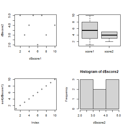
In this data exploration phase it is very useful to make plots. We’ll
discuss plotting in a later chapter, but here are four example plots.
Note how par(mfrow=c(2,2)) sets up the canvas for two rows and
columns, that is for four plots.
par(mfrow=c(2,2))
plot(d$score1, d$score2)
boxplot(d[, c("score1", "score2")])
plot(sort(d$score1))
hist(d$score2)