Statistical models
There are many type of statistical models. Here we show how to make simple regression models with R. Other modeling approaches tend to use similar syntax.
The most common way to specify a regression model in R is by creating
a formula. For example y ~ x means y is a function of x.
y ~ a + b means that y is a function of a and b.
Let’s use the cars data that come with R. This dataset has
measurements on the distance needed to stop given the speed a car was
driven when the driver stepped on the breaks. We use the lm (linear
model) function.
head(cars)
##   speed dist
## 1     4    2
## 2     4   10
## 3     7    4
## 4     7   22
## 5     8   16
## 6     9   10
m <- lm(dist ~ speed, data=cars)
m
##
## Call:
## lm(formula = dist ~ speed, data = cars)
##
## Coefficients:
## (Intercept)        speed
##     -17.579        3.932
Note that the data is provided by data.frame cars, and that the
names in formula are column names in this data.frame. The functions
returned a model (lm) object. When printed it shows the coefficients
of the regression model (dist = -17.579 + 3.932 * speed). m has
quite a bit more information, but that is not shown, by default.
There are several functions that can be used to extract this information.
summary(m)
##
## Call:
## lm(formula = dist ~ speed, data = cars)
##
## Residuals:
##     Min      1Q  Median      3Q     Max
## -29.069  -9.525  -2.272   9.215  43.201
##
## Coefficients:
##             Estimate Std. Error t value Pr(>|t|)
## (Intercept) -17.5791     6.7584  -2.601   0.0123 *
## speed         3.9324     0.4155   9.464 1.49e-12 ***
## ---
## Signif. codes:  0 '***' 0.001 '**' 0.01 '*' 0.05 '.' 0.1 ' ' 1
##
## Residual standard error: 15.38 on 48 degrees of freedom
## Multiple R-squared:  0.6511, Adjusted R-squared:  0.6438
## F-statistic: 89.57 on 1 and 48 DF,  p-value: 1.49e-12
anova(m)
## Analysis of Variance Table
##
## Response: dist
##           Df Sum Sq Mean Sq F value   Pr(>F)
## speed      1  21186 21185.5  89.567 1.49e-12 ***
## Residuals 48  11354   236.5
## ---
## Signif. codes:  0 '***' 0.001 '**' 0.01 '*' 0.05 '.' 0.1 ' ' 1
residuals(m)[1:10]
##         1         2         3         4         5         6         7         8
##  3.849460 11.849460 -5.947766 12.052234  2.119825 -7.812584 -3.744993  4.255007
##         9        10
## 12.255007 -8.677401
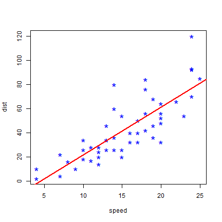
You can use abline to draw a simple regression line like this.
plot(cars, col='blue', pch='*', cex=2)
abline(m, col='red', lwd=2)
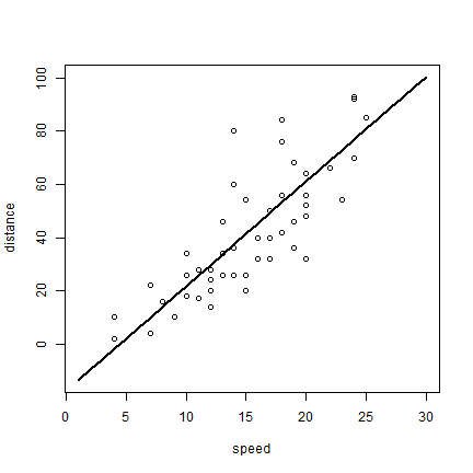
More generally, you can use the predict function to use the model to
predict values of y for any x.
p <- predict(m, data.frame(speed=1:30))
p
##          1          2          3          4          5          6          7
## -13.646686  -9.714277  -5.781869  -1.849460   2.082949   6.015358   9.947766
##          8          9         10         11         12         13         14
##  13.880175  17.812584  21.744993  25.677401  29.609810  33.542219  37.474628
##         15         16         17         18         19         20         21
##  41.407036  45.339445  49.271854  53.204263  57.136672  61.069080  65.001489
##         22         23         24         25         26         27         28
##  68.933898  72.866307  76.798715  80.731124  84.663533  88.595942  92.528350
##         29         30
##  96.460759 100.393168
plot(1:30, p, xlab='speed', ylab='distance', type='l', lwd=2)
points(cars)
The glm (generalized linear models) function can do what lm can,
but it is much more versatile. For example you can also use it for
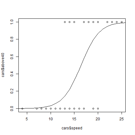
logistic regression. In logistic regression the response variable is
normally binomial (0 or 1) or at least between 0 and 1. I create such a
variable here (was the stopping distance above 40 or not?).
cars$above40 <- cars$dist > 40
Now we can use this variable in a glm model. By stating that
family='binomial' we indicate that we want logistic regression. (The
default is family=gaussian which indicates standard (normal)
regression.
mlog <- glm(above40 ~ speed, data=cars, family='binomial')
mlog
##
## Call:  glm(formula = above40 ~ speed, family = "binomial", data = cars)
##
## Coefficients:
## (Intercept)        speed
##      -8.553        0.521
##
## Degrees of Freedom: 49 Total (i.e. Null);  48 Residual
## Null Deviance:       68.59
## Residual Deviance: 36.37     AIC: 40.37
Because a logistic model operates with logistically transformed numbers,
we need to tell the predict function that we want the predicted values
on the original scale (type='response').
p <- predict(mlog, data.frame(speed=1:30), type='response')
plot(cars$speed, cars$above40)
lines(1:30, p)