Spatial regression models
Introduction
This chapter deals with the problem of inference in (regression) models with spatial data. Inference from regression models with spatial data can be suspect. In essence this is because nearby things are similar, and it may not be fair to consider individual cases as independent (they may be pseudo-replicates). Therefore, such models need to be diagnosed before reporting them. Specifically, it is important to evaluate the for spatial autocorrelation in the residuals (as these are supposed to be independent, not correlated). If the residuals are spatially autocorrelated, this indicates that the model is misspecified. In that case you should try to improve the model by adding (and perhaps removing) important variables. If that is not possible (either because there is no data available, or because you have no clue as to what variable to look for), you can try formulating a regression model that controls for spatial autocorrelation. We show some examples of that approach here.
Reading & aggregating data
We use California house price data from the 2000 Census.
Get the data
if (!require("rspatial")) remotes::install_github('rspatial/rspatial')
library(rspatial)
h <- sp_data('houses2000')
I have selected some variables on on housing and population. You can get more data from the American Fact Finder http://factfinder2.census.gov (among other web sites).
library(raster)
dim(h)
## [1] 7049   29
names(h)
##  [1] "TRACT"      "GEOID"      "label"      "houseValue" "nhousingUn"
##  [6] "recHouses"  "nMobileHom" "yearBuilt"  "nBadPlumbi" "nBadKitche"
## [11] "nRooms"     "nBedrooms"  "medHHinc"   "Population" "Males"
## [16] "Females"    "Under5"     "MedianAge"  "White"      "Black"
## [21] "AmericanIn" "Asian"      "Hispanic"   "PopInHouse" "nHousehold"
## [26] "Families"   "householdS" "familySize" "County"
These are the variables we have:
variable | explanation |
nhousingUn | number of housing units |
recHouses | number of houses for recreational use |
nMobileHom | number of mobile homes |
nBadPlumbi | number of houses with incomplete plumbing |
nBadKitche | number of houses with incomplete kitchens |
Population | total population |
Males | number of males |
Females | number of females |
Under5 | number of persons under five |
White | number of persons identifying themselves as white (only) |
Black | number of persons identifying themselves African-american (only) |
AmericanIn | number of persons identifying themselves American Indian (only) |
Asian | number of persons identifying themselves as American Indian (only) |
Hispanic | number of persons identifying themselves as hispanic (only) |
PopInHouse | number of persons living in households |
nHousehold | number of households |
Families | number of families |
houseValue | value of the house |
yearBuilt | year house was built |
nRooms | median number of rooms per house |
nBedrooms | median number of bedrooms per house |
medHHinc | median household income |
MedianAge | median age of population |
householdS | median household size |
familySize | median family size |
First some data massaging. These are values for Census tracts. I want to analyze these data at the county level. So we need to aggregate the values.
hh <- aggregate(h, "County")
## Warning in RGEOSUnaryPredFunc(spgeom, byid, "rgeos_isvalid"): Ring Self-
## intersection at or near point -116.530348 33.743321000000002
## Warning in RGEOSUnaryPredFunc(spgeom, byid, "rgeos_isvalid"): Ring Self-
## intersection at or near point -116.56294699999999 33.844917000000002
## z is invalid
## Warning in gBuffer(spgeom, byid = TRUE, width = 0): Spatial object is not
## projected; GEOS expects planar coordinates
## Attempting to make z valid by zero-width buffering
Now we have the county outlines, but we also need to get the values of interest at the county level. Although it is possible to do everything in one step in the aggregate function, I prefer to do this step by step. The simplest case is where we can sum the numbers. For example for the number of houses.
d1 <- data.frame(h)[, c("nhousingUn", "recHouses", "nMobileHom", "nBadPlumbi",
 "nBadKitche", "Population", "Males", "Females", "Under5", "White",
 "Black", "AmericanIn", "Asian", "Hispanic", "PopInHouse", "nHousehold", "Families")]
 d1a <- aggregate(d1, list(County=h$County), sum, na.rm=TRUE)
In other cases we need to use a weighted mean. For example for houseValue
d2 <- data.frame(h)[, c("houseValue", "yearBuilt", "nRooms", "nBedrooms",
       "medHHinc", "MedianAge", "householdS",  "familySize")]
d2 <- cbind(d2 * h$nHousehold, hh=h$nHousehold)
d2a <- aggregate(d2, list(County=h$County), sum, na.rm=TRUE)
d2a[, 2:ncol(d2a)] <- d2a[, 2:ncol(d2a)] / d2a$hh
Combine these two groups:
d12 <- merge(d1a, d2a, by='County')
And merge the aggregated (from census tract to county level) attribute data with the aggregated polygons
hh <- merge(hh, d12, by='County')
Let’s make some maps, at the orignal Census tract level. We are using a bit more advanced (and slower) plotting methods here. First the house value, using a legend with 10 intervals.
library(latticeExtra)
## Loading required package: lattice
library(RColorBrewer)
grps <- 10
brks <- quantile(h$houseValue, 0:(grps-1)/(grps-1), na.rm=TRUE)
p <- spplot(h, "houseValue", at=brks, col.regions=rev(brewer.pal(grps, "RdBu")), col="transparent" )
p + layer(sp.polygons(hh))
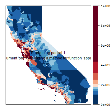
This takes very long. spplot (levelplot) is a bit slow when using a large dataset…
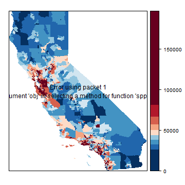
A map of the median household income.
brks <- quantile(h$medHHinc, 0:(grps-1)/(grps-1), na.rm=TRUE)
p <- spplot(h, "medHHinc", at=brks, col.regions=rev(brewer.pal(grps, "RdBu")), col="transparent")
p + layer(sp.polygons(hh))
Basic OLS model
I’ll now make some models with the county-level data. I first compute some new variables (that I might not all use).
hh$fBadP <- pmax(hh$nBadPlumbi, hh$nBadKitche) / hh$nhousingUn
hh$fWhite <- hh$White / hh$Population
hh$age <- 2000 - hh$yearBuilt
f1 <- houseValue ~ age +  nBedrooms
m1 <- lm(f1, data=hh)
summary(m1)
##
## Call:
## lm(formula = f1, data = hh)
##
## Residuals:
##     Min      1Q  Median      3Q     Max
## -222541  -67489   -6128   60509  217655
##
## Coefficients:
##             Estimate Std. Error t value Pr(>|t|)
## (Intercept)  -628578     233217  -2.695  0.00931 **
## age            12695       2480   5.119 4.05e-06 ***
## nBedrooms     191889      76756   2.500  0.01543 *
## ---
## Signif. codes:  0 '***' 0.001 '**' 0.01 '*' 0.05 '.' 0.1 ' ' 1
##
## Residual standard error: 94740 on 55 degrees of freedom
## Multiple R-squared:  0.3235, Adjusted R-squared:  0.2989
## F-statistic: 13.15 on 2 and 55 DF,  p-value: 2.147e-05
Just for illustration, here is how you can do OLS with matrix algebra. First set up the data. I add a constant variable ‘1’ to X, to get an intercept.
y <- matrix(hh$houseValue)
X <- cbind(1, hh$age, hh$nBedrooms)
Then use matrix algebra
ols <- solve(t(X) %*% X) %*% t(X) %*% y
rownames(ols) <- c('intercept', 'age', 'nBedroom')
ols
##                 [,1]
## intercept -628577.95
## age         12694.75
## nBedroom   191888.89
So, according to this simple model, “age” is highly significant. The older a house, the more expensive. You pay 1,269,475 dollars more for a house that is 100 years old than a for new house! While the p-value for the number of bedrooms is not impressive, but every bedroom adds about 200,000 dollars to the value of a house.
Question 1: What would be the price be of a house built in 1999 with three bedrooms?
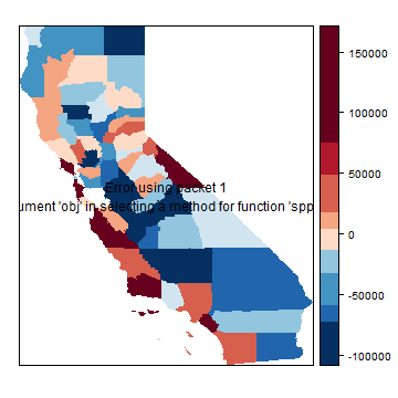
Let’s see if the errors (model residuals) appear to be randomly distributed in space.
hh$residuals <- residuals(m1)
brks <- quantile(hh$residuals, 0:(grps-1)/(grps-1), na.rm=TRUE)
spplot(hh, "residuals", at=brks, col.regions=rev(brewer.pal(grps, "RdBu")), col="black")
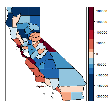
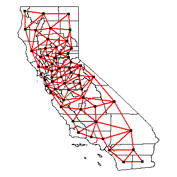
What do think? Is this random? Let’s see what Mr. Moran would say. First make a neighborhoods list. I add two links: between San Francisco and Marin County and vice versa (to consider the Golden Gate bridge).
library(spdep)
nb <- poly2nb(hh)
nb[[21]] <- sort(as.integer(c(nb[[21]], 38)))
nb[[38]] <- sort(as.integer(c(21, nb[[38]])))
nb
## Neighbour list object:
## Number of regions: 58
## Number of nonzero links: 278
## Percentage nonzero weights: 8.263971
## Average number of links: 4.793103
par(mai=c(0,0,0,0))
plot(hh)
plot(nb, coordinates(hh), col='red', lwd=2, add=TRUE)
We can use the neighbour list object to get the average value for the neighbors of each polygon.
resnb <- sapply(nb, function(x) mean(hh$residuals[x]))
cor(hh$residuals, resnb)
## [1] 0.6311218
plot(hh$residuals, resnb, xlab='Residuals', ylab='Mean adjacent residuals')
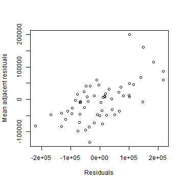
lw <- nb2listw(nb)
That does not look independent.
moran.mc(hh$residuals, lw, 999)
##
##  Monte-Carlo simulation of Moran I
##
## data:  hh$residuals
## weights: lw
## number of simulations + 1: 1000
##
## statistic = 0.41428, observed rank = 1000, p-value = 0.001
## alternative hypothesis: greater
Clearly, there is spatial autocorrelation. Our p-values and regression model coefficients cannot be trusted. so let’s try SAR models.
Spatial lag model
Here I show a how to do spatial regression with a spatial lag model
(lagsarlm), using the spatialreg package.
library(spatialreg )
m1s = lagsarlm(f1, data=hh, lw, tol.solve=1.0e-30)
summary(m1s)
##
## Call:lagsarlm(formula = f1, data = hh, listw = lw, tol.solve = 1e-30)
##
## Residuals:
##       Min        1Q    Median        3Q       Max
## -108145.2  -49816.3   -1316.3   44604.9  171536.0
##
## Type: lag
## Coefficients: (asymptotic standard errors)
##              Estimate Std. Error z value Pr(>|z|)
## (Intercept) -418674.1   153693.6 -2.7241 0.006448
## age            5533.6     1698.2  3.2584 0.001120
## nBedrooms    127912.8    50859.7  2.5150 0.011903
##
## Rho: 0.77413, LR test value: 34.761, p-value: 3.7282e-09
## Asymptotic standard error: 0.08125
##     z-value: 9.5277, p-value: < 2.22e-16
## Wald statistic: 90.778, p-value: < 2.22e-16
##
## Log likelihood: -727.9964 for lag model
## ML residual variance (sigma squared): 3871700000, (sigma: 62223)
## Number of observations: 58
## Number of parameters estimated: 5
## AIC: 1466, (AIC for lm: 1498.8)
## LM test for residual autocorrelation
## test value: 0.12431, p-value: 0.72441
hh$residuals <- residuals(m1s)
moran.mc(hh$residuals, lw, 999)
##
##  Monte-Carlo simulation of Moran I
##
## data:  hh$residuals
## weights: lw
## number of simulations + 1: 1000
##
## statistic = -0.016, observed rank = 509, p-value = 0.491
## alternative hypothesis: greater
brks <- quantile(hh$residuals, 0:(grps-1)/(grps-1), na.rm=TRUE)
p <- spplot(hh, "residuals", at=brks, col.regions=rev(brewer.pal(grps, "RdBu")), col="transparent")
print( p + layer(sp.polygons(hh)) )
Spatial error model
And now with a “Spatial error” (or spatial moving average) models (errorsarlm)
m1e <- errorsarlm(f1, data=hh, lw, tol.solve=1.0e-30)
summary(m1e)
##
## Call:errorsarlm(formula = f1, data = hh, listw = lw, tol.solve = 1e-30)
##
## Residuals:
##       Min        1Q    Median        3Q       Max
## -100640.7  -47783.1   -2364.5   44180.6  181876.5
##
## Type: error
## Coefficients: (asymptotic standard errors)
##              Estimate Std. Error z value Pr(>|z|)
## (Intercept) -185443.8   180133.7 -1.0295  0.30325
## age            4313.6     2214.9  1.9475  0.05147
## nBedrooms    117864.4    51564.7  2.2858  0.02227
##
## Lambda: 0.82151, LR test value: 29.781, p-value: 4.8373e-08
## Asymptotic standard error: 0.071111
##     z-value: 11.552, p-value: < 2.22e-16
## Wald statistic: 133.46, p-value: < 2.22e-16
##
## Log likelihood: -730.4863 for error model
## ML residual variance (sigma squared): 4.07e+09, (sigma: 63797)
## Number of observations: 58
## Number of parameters estimated: 5
## AIC: 1471, (AIC for lm: 1498.8)
hh$residuals <- residuals(m1e)
moran.mc(hh$residuals, lw, 999)
##
##  Monte-Carlo simulation of Moran I
##
## data:  hh$residuals
## weights: lw
## number of simulations + 1: 1000
##
## statistic = 0.039033, observed rank = 743, p-value = 0.257
## alternative hypothesis: greater
brks <- quantile(hh$residuals, 0:(grps-1)/(grps-1), na.rm=TRUE)
p <- spplot(hh, "residuals", at=brks, col.regions=rev(brewer.pal(grps, "RdBu")),
 col="transparent")
print( p + layer(sp.polygons(hh)) )
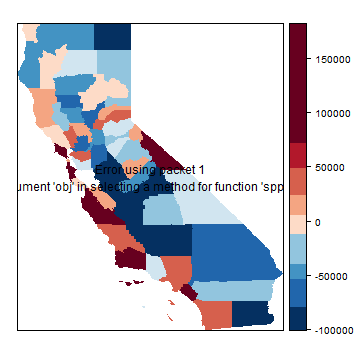
Are the residuals spatially autocorrelated for either of these models? Let’s plot them for the spatial error model.
brks <- quantile(hh$residuals, 0:(grps-1)/(grps-1), na.rm=TRUE)
p <- spplot(hh, "residuals", at=brks, col.regions=rev(brewer.pal(grps, "RdBu")),
 col="transparent")
print( p + layer(sp.polygons(hh)) )

Questions
Question 2: The last two maps still seem to show a lot of spatial autocorrelation. But according to the tests there is none. Now why might that be?
Question 3: One of the most important, or perhaps THE most important aspect of modeling is variable selection. A misspecified model is never going to be any good, no matter how much you do to, e.g., correct for spatial autocorrelation.
Which variables would you choose from the list?
Which new variables could you propose to create from the variables in the list.
Which other variables could you add, created from the geometries/location (perhaps other geographic data).
add a lot of variables and use stepAIC to select an ‘optimal’ OLS model
check for spatial autocorrelation in the residuals of that model