Spatial autocorrelation
Introduction
Spatial autocorrelation is an important concept in spatial statistics. It is a both a nuisance, as it complicates statistical tests, and a feature, as it allows for spatial interpolation. Its computation and properties are often misunderstood. This chapter discusses what it is, and how statistics describing it can be computed.
Autocorrelation (whether spatial or not) is a measure of similarity (correlation) between nearby observations. To understand spatial autocorrelation, it helps to first consider temporal autocorrelation.
Temporal autocorrelation
If you measure something about the same object over time, for example a persons weight or wealth, it is likely that two observations that are close to each other in time are also similar in measurement. Say that over a couple of years your weight went from 50 to 80 kg. It is unlikely that it was 60 kg one day, 50 kg the next and 80 the day after that. Rather it probably went up gradually, with the occasional tapering off, or even reverse in direction. The same may be true with your bank account, but that may also have a marked monthly trend. To measure the degree of association over time, we can compute the correlation of each observation with the next observation.
Let d be a vector of daily observations.
set.seed(0)
d <- sample(100, 10)
d
##  [1]  14  68  39   1  34  87  43 100  82  59
Compute auto-correlation.
a <- d[-length(d)]
b <- d[-1]
plot(a, b, xlab='t', ylab='t-1')
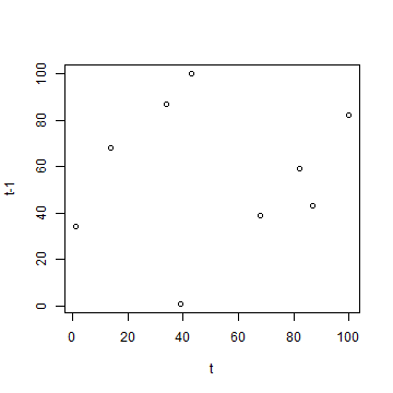
cor(a, b)
## [1] 0.1227634
The autocorrelation computed above is very small. Even though this is a random sample, you (almost) never get a value of zero. We computed the “one-lag” autocorrelation, that is, we compare each value to its immediate neighbour, and not to other nearby values.
After sorting the numbers in d autocorrelation becomes very strong
(unsurprisingly).
d <- sort(d)
d
##  [1]   1  14  34  39  43  59  68  82  87 100
a <- d[-length(d)]
b <- d[-1]
plot(a, b, xlab='t', ylab='t-1')
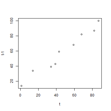
cor(a, b)
## [1] 0.9819258
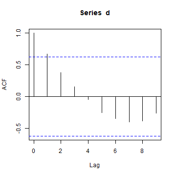
The acf function shows autocorrelation computed in a slightly
different
way
for several lags (it is 1 to each point it self, very high when
comparing with the nearest neighbour, and than tapering off).
acf(d)
Spatial autocorrelation
The concept of spatial autocorrelation is an extension of temporal autocorrelation. It is a bit more complicated though. Time is one-dimensional, and only goes in one direction, ever forward. Spatial objects have (at least) two dimensions and complex shapes, and it may not be obvious how to determine what is “near”.
Measures of spatial autocorrelation describe the degree two which observations (values) at spatial locations (whether they are points, areas, or raster cells), are similar to each other. So we need two things: observations and locations.
Spatial autocorrelation in a variable can be exogenous (it is caused by another spatially autocorrelated variable, e.g. rainfall) or endogenous (it is caused by the process at play, e.g. the spread of a disease).
A commonly used statistic that describes spatial autocorrelation is Moran’s I, and we’ll discuss that here in detail. Other indices include Geary’s C and, for binary data, the join-count index. The semi-variogram also expresses the amount of spatial autocorrelation in a data set (see the chapter on interpolation).
Example data
Read the example data
library(raster)
p <- shapefile(system.file("external/lux.shp", package="raster"))
p <- p[p$NAME_1=="Diekirch", ]
p$value <- c(10, 6, 4, 11, 6)
data.frame(p)
##   ID_1   NAME_1 ID_2   NAME_2 AREA value
## 0    1 Diekirch    1 Clervaux  312    10
## 1    1 Diekirch    2 Diekirch  218     6
## 2    1 Diekirch    3  Redange  259     4
## 3    1 Diekirch    4  Vianden   76    11
## 4    1 Diekirch    5    Wiltz  263     6
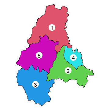
Let’s say we are interested in spatial autocorrelation in variable “AREA”. If there were spatial autocorrelation, regions of a similar size would be spatially clustered.
Here is a plot of the polygons. I use the coordinates function to
get the centroids of the polygons to place the labels.
par(mai=c(0,0,0,0))
plot(p, col=2:7)
xy <- coordinates(p)
points(xy, cex=6, pch=20, col='white')
text(p, 'ID_2', cex=1.5)
Adjacent polygons
Now we need to determine which polygons are “near”, and how to quantify that. Here we’ll use adjacency as criterion. To find adjacent polygons, we can use package ‘spdep’.
library(spdep)
w <- poly2nb(p, row.names=p$Id)
class(w)
## [1] "nb"
summary(w)
## Neighbour list object:
## Number of regions: 5
## Number of nonzero links: 14
## Percentage nonzero weights: 56
## Average number of links: 2.8
## Link number distribution:
##
## 2 3 4
## 2 2 1
## 2 least connected regions:
## 2 3 with 2 links
## 1 most connected region:
## 1 with 4 links
summary(w) tells us something about the neighborhood. The average
number of neighbors (adjacent polygons) is 2.8, 3 polygons have 2
neighbors and 1 has 4 neighbors (which one is that?).
For more details we can look at the structure of w.
str(w)
## List of 5
##  $ : int [1:3] 2 4 5
##  $ : int [1:4] 1 3 4 5
##  $ : int [1:2] 2 5
##  $ : int [1:2] 1 2
##  $ : int [1:3] 1 2 3
##  - attr(*, "class")= chr "nb"
##  - attr(*, "region.id")= chr [1:5] "0" "1" "2" "3" ...
##  - attr(*, "call")= language poly2nb(pl = p, row.names = p$Id)
##  - attr(*, "type")= chr "queen"
##  - attr(*, "sym")= logi TRUE
Question 1:Explain the meaning of the first 5 lines returned by str(w)
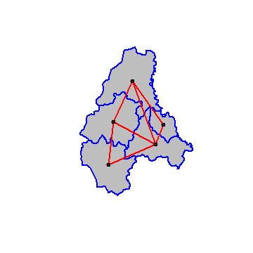
Plot the links between the polygons.
plot(p, col='gray', border='blue', lwd=2)
plot(w, xy, col='red', lwd=2, add=TRUE)
We can transform w into a spatial weights matrix. A spatial weights
matrix reflects the intensity of the geographic relationship between
observations (see previous chapter).
wm <- nb2mat(w, style='B')
wm
##   [,1] [,2] [,3] [,4] [,5]
## 0    0    1    0    1    1
## 1    1    0    1    1    1
## 2    0    1    0    0    1
## 3    1    1    0    0    0
## 4    1    1    1    0    0
## attr(,"call")
## nb2mat(neighbours = w, style = "B")
Compute Moran’s I
Now let’s compute Moran’s index of spatial autocorrelation
Yes, that looks impressive. But it is not much more than an expanded version of the formula to compute the correlation coefficient. The main thing that was added is the spatial weights matrix.
The number of observations
n <- length(p)
Get ‘y’ and ‘ybar’ (the mean value of y)
y <- p$value
ybar <- mean(y)
Now we need
That is, (yi-ybar)(yj-ybar) for all pairs. I show two methods to get that.
Method 1:
dy <- y - ybar
g <- expand.grid(dy, dy)
yiyj <- g[,1] * g[,2]
Method 2:
yi <- rep(dy, each=n)
yj <- rep(dy)
yiyj <- yi * yj
Make a matrix of the multiplied pairs
pm <- matrix(yiyj, ncol=n)
And multiply this matrix with the weights to set to zero the value for the pairs that are not adjacent.
pmw <- pm * wm
pmw
##    [,1]  [,2] [,3]  [,4]  [,5]
## 0  0.00 -3.64 0.00  9.36 -3.64
## 1 -3.64  0.00 4.76 -5.04  1.96
## 2  0.00  4.76 0.00  0.00  4.76
## 3  9.36 -5.04 0.00  0.00  0.00
## 4 -3.64  1.96 4.76  0.00  0.00
## attr(,"call")
## nb2mat(neighbours = w, style = "B")
We now sum the values, to get this bit of Moran’s I:
spmw <- sum(pmw)
spmw
## [1] 17.04
The next step is to divide this value by the sum of weights. That is easy.
smw <- sum(wm)
sw  <- spmw / smw
And compute the inverse variance of y
vr <- n / sum(dy^2)
The final step to compute Moran’s I
MI <- vr * sw
MI
## [1] 0.1728896
This is a simple (but crude) way to estimate the expected value of Moran’s I. That is, the value you would get in the absence of spatial autocorelation (if the data were spatially random). Of course you never really expect that, but that is how we do it in statistics. Note that the expected value approaches zero if n becomes large, but that it is not quite zero for small values of n.
EI <- -1/(n-1)
EI
## [1] -0.25
After doing this ‘by hand’, now let’s use the spdep package to compute Moran’s I and do a significance test. To do this we need to create a ‘listw’ type spatial weights object (instead of the matrix we used above). To get the same value as above we use “style=‘B’” to use binary (TRUE/FALSE) distance weights.
ww <-  nb2listw(w, style='B')
ww
## Characteristics of weights list object:
## Neighbour list object:
## Number of regions: 5
## Number of nonzero links: 14
## Percentage nonzero weights: 56
## Average number of links: 2.8
##
## Weights style: B
## Weights constants summary:
##   n nn S0 S1  S2
## B 5 25 14 28 168
Now we can use the moran function. Have a look at ?moran. The
function is defined as ‘moran(y, ww, n, Szero(ww))’. Note the odd
arguments n and S0. I think they are odd, because “ww” has that
information. Anyway, we supply them and it works. There probably are
cases where it makes sense to use other values.
moran(p$value, ww, n=length(ww$neighbours), S0=Szero(ww))
## $I
## [1] 0.1728896
##
## $K
## [1] 1.432464
#Note that
Szero(ww)
## [1] 14
# is the same as
pmw
##    [,1]  [,2] [,3]  [,4]  [,5]
## 0  0.00 -3.64 0.00  9.36 -3.64
## 1 -3.64  0.00 4.76 -5.04  1.96
## 2  0.00  4.76 0.00  0.00  4.76
## 3  9.36 -5.04 0.00  0.00  0.00
## 4 -3.64  1.96 4.76  0.00  0.00
## attr(,"call")
## nb2mat(neighbours = w, style = "B")
sum(pmw==0)
## [1] 11
Now we can test for significance. First analytically, using linear regression based logic and assumptions.
moran.test(p$value, ww, randomisation=FALSE)
##
##  Moran I test under normality
##
## data:  p$value
## weights: ww
##
## Moran I statistic standard deviate = 2.3372, p-value = 0.009714
## alternative hypothesis: greater
## sample estimates:
## Moran I statistic       Expectation          Variance
##         0.1728896        -0.2500000         0.0327381
Instead of the approach above you should use Monte Carlo simulation. That is the preferred method (in fact, the only good method). The oay it works that the values are randomly assigned to the polygons, and the Moran’s I is computed. This is repeated several times to establish a distribution of expected values. The observed value of Moran’s I is then compared with the simulated distribution to see how likely it is that the observed values could be considered a random draw.
moran.mc(p$value, ww, nsim=99)
##
##  Monte-Carlo simulation of Moran I
##
## data:  p$value
## weights: ww
## number of simulations + 1: 100
##
## statistic = 0.17289, observed rank = 98, p-value = 0.02
## alternative hypothesis: greater
Question 2: How do you interpret these results (the significance tests)?
Also try this code, it gives an error:
moran.mc(p$value, ww, nsim=999)
Question 3: What is the maximum value we can use for nsim?
We can make a “Moran scatter plot” to visualize spatial autocorrelation. We first get the neighbouring values for each value.
n <- length(p)
ms <- cbind(id=rep(1:n, each=n), y=rep(y, each=n), value=as.vector(wm * y))
Remove the zeros
ms <- ms[ms[,3] > 0, ]
And compute the average neighbour value
ams <- aggregate(ms[,2:3], list(ms[,1]), FUN=mean)
ams <- ams[,-1]
colnames(ams) <- c('y', 'spatially lagged y')
head(ams)
##    y spatially lagged y
## 1 10           7.666667
## 2  6           7.750000
## 3  4           6.000000
## 4 11           8.000000
## 5  6           6.666667
Finally, the plot.
plot(ams)
reg <- lm(ams[,2] ~ ams[,1])
abline(reg, lwd=2)
abline(h=mean(ams[,2]), lt=2)
abline(v=ybar, lt=2)
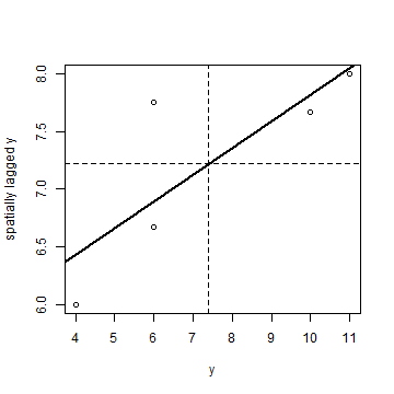
Note that the slope of the regression line:
coefficients(reg)[2]
##  ams[, 1]
## 0.2315341
is almost the same as Moran’s I.
Here is a more direct approach to accomplish the same thing (but hopefully the above makes it clearer how this is actually computed). Note the row standardisation of the weights matrix:
rwm <- mat2listw(wm, style='W')
# Checking if rows add up to 1
mat <- listw2mat(rwm)
apply(mat, 1, sum)[1:15]
##    0    1    2    3    4 <NA> <NA> <NA> <NA> <NA> <NA> <NA> <NA> <NA> <NA>
##    1    1    1    1    1   NA   NA   NA   NA   NA   NA   NA   NA   NA   NA
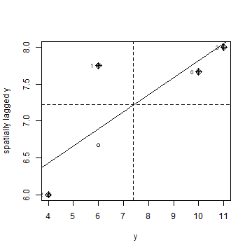
Now we can plot
moran.plot(y, rwm)
Question 4: Show how to use the ‘geary’ function to compute Geary’s C
Question 5: Write your own Monte Carlo simulation test to compute p-values for Moran’s I, replicating the results we obtained with the function from spdep. Show a histogram of the simulated values.
Question 6: Write your own Geary C function, by completing the function below
gearyC <- ((n-1)/sum(( "----")\^2)) * sum(wm * (" --- ")\^2) / (2 * sum(wm))