Spatial distribution models¶

This page shows how you can use the Random Forest algorithm to make spatial predictions. This approach is widely used, for example to classify remote sensing data into different land cover classes. But here our objective is to predict the entire range of a species based on a set of locations where it has been observed. As an example, we use the hominid species Imaginus magnapedum (also known under the vernacular names of “bigfoot” and “sasquatch”). This species is so hard to find (at least by scientists) that its very existence is commonly denied by the mainstream media! For more information about this controversy, see the article by Lozier, Aniello and Hickerson: Predicting the distribution of Sasquatch in western North America: anything goes with ecological niche modelling.

We want to find out

What the complete range of the species might be.
How good (general) our model is by predicting the range of the Eastern sub-species, with data from the Western sub-species.
Predict where in Mexico the creature is likely to occur.
How climate change might affect its distribution.

In this context, this type of analysis is often referred to as ‘species distribution modeling’ or ‘ecological niche modeling’. Here is a more in-depth discussion of this technique.

Data¶

Observations¶

if (!require("rspatial")) remotes::install_github('rspatial/rspatial')
library(rspatial)
bf <- sp_data('bigfoot')
dim(bf)
## [1] 3092    3
head(bf)
##         lon      lat Class
## 1 -142.9000 61.50000     A
## 2 -132.7982 55.18720     A
## 3 -132.8202 55.20350     A
## 4 -141.5667 62.93750     A
## 5 -149.7853 61.05950     A
## 6 -141.3165 62.77335     A

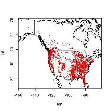
Plot the locations

plot(bf[,1:2], cex=0.5, col='red')
library(maptools)
## Checking rgeos availability: TRUE
## Please note that 'maptools' will be retired by the end of 2023,
## plan transition at your earliest convenience;
## some functionality will be moved to 'sp'.
data(wrld_simpl)
plot(wrld_simpl, add=TRUE)

Predictors¶

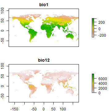
Supervised classification often uses predictor data obtained from satellite remote sensing. But here, as is common in species distribution modeling, we use climate data. Specifically, we use ‘bioclimatic variables’, see: http://www.worldclim.org/bioclim

library(raster)
wc <- raster::getData('worldclim', res=10, var='bio')
plot(wc[[c(1, 12)]], nr=2)

Now extract climate data for the locations of our observations. That is, get data about the climate that the species likes, apparently.

bfc <- extract(wc, bf[,1:2])
head(bfc)
##      bio1 bio2 bio3  bio4 bio5 bio6 bio7 bio8 bio9 bio10 bio11 bio12 bio13
## [1,]  -14  102   27  9672  174 -197  371   51  -11   108  -137   973   119
## [2,]   62   55   31  4136  157  -17  174   43   98   118    15  2602   385
## [3,]   62   55   31  4136  157  -17  174   43   98   118    15  2602   385
## [4,]  -57  125   23 15138  206 -332  538  127 -129   127  -256   282    67
## [5,]   10   80   25  8308  174 -140  314   66    5   119   -91   532    81
## [6,]  -59  128   23 14923  204 -334  538  122 -130   122  -255   322    75
##      bio14 bio15 bio16 bio17 bio18 bio19
## [1,]    43    30   332   156   290   210
## [2,]   128    33   953   407   556   721
## [3,]   128    33   953   407   556   721
## [4,]     6    81   163    22   163    27
## [5,]    22    41   215    72   159   117
## [6,]     8    79   183    28   183    32
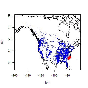
# Any missing values?
i <- which(is.na(bfc[,1]))
i
## [1]  862 2667
plot(bf[,1:2], cex=0.5, col='blue')
plot(wrld_simpl, add=TRUE)
points(bf[i, ], pch=20, cex=3, col='red')

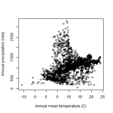
Here is a plot that illustrates a component of the ecological niche of our species of interest.

plot(bfc[ ,'bio1'] / 10, bfc[, 'bio12'], xlab='Annual mean temperature (C)',
         ylab='Annual precipitation (mm)')

Background data¶

Normally, one would build a model that would compare the values of the predictor variables as the locations where something was observed, with those values at the locations where it was not observed. But we do not have data from a systematic survey that determined presence and absence. We have presence-only data. (And, determining absence is not that simple. It is here now, it is gone tomorrow).

The common trick to deal with this is to not model presence versus absence, but presence versus a ‘random expectation’. This random expectation (also referred to as ‘background’, or ‘random-absence’ data) is what you would get if the species had no preference for any of the predictor variables (or to other variables that are not in the model, but correlated with the predictor variables).

There is not much point in taking absence data from very far away (tropical Africa or Antarctica). Typically they are taken from more or less the entire study area for which we have presences data.

library(dismo)
# extent of all points
e <- extent(SpatialPoints(bf[, 1:2]))
e
## class      : Extent
## xmin       : -156.75
## xmax       : -64.4627
## ymin       : 25.141
## ymax       : 69.5
# 5000 random samples (excluding NA cells) from extent e
set.seed(0)
bg <- sampleRandom(wc, 5000, ext=e)
dim(bg)
## [1] 5000   19
head(bg)
##      bio1 bio2 bio3  bio4 bio5 bio6 bio7 bio8 bio9 bio10 bio11 bio12 bio13
## [1,]  157  126   60  2935  262   55  207  124  191   197   122   379    88
## [2,]  -54  105   28  9244  142 -223  365   57  -62    68  -165   639    79
## [3,]  -57  104   20 14227  198 -317  515  106 -227   118  -247   473    71
## [4,]    1  119   24 12335  231 -251  482  138  -91   150  -168   844   104
## [5,]  208  169   44  7641  404   28  376  304  239   307   114   198    31
## [6,]  -89  111   23 12931  160 -316  476   78 -174    78  -248   476    76
##      bio14 bio15 bio16 bio17 bio18 bio19
## [1,]     0   100   225     2     4   222
## [2,]    28    30   226   101   219   138
## [3,]    17    46   197    55   194    59
## [4,]    34    33   301   128   291   137
## [5,]     2    50    73    11    52    62
## [6,]    25    40   193    79   193    82

Combine presence and background¶

d <- rbind(cbind(pa=1, bfc), cbind(pa=0, bg))
d <- data.frame(d)
dim(d)
## [1] 8092   20

Fit a model¶

Now we have the data to fit a model. But I am going to split the data into East and West. Let’s say I believe these are actually are different, albeit related, sub-species (The Eastern Sasquatch is darker and less hairy). I am principally interested in the western sub-species.

de <- d[bf[,1] > -102, ]
dw <- d[bf[,1] <= -102, ]

CART¶

Let’s first look at a Classification and Regression Trees (CART) model.

library(rpart)
cart <- rpart(pa~., data=dw)
printcp(cart)
##
## Regression tree:
## rpart(formula = pa ~ ., data = dw)
##
## Variables actually used in tree construction:
## [1] bio10 bio14 bio15 bio18 bio3  bio4  bio5  bio6  bio8
##
## Root node error: 762.45/3246 = 0.23489
##
## n= 3246
##
##         CP nsplit rel error  xerror     xstd
## 1 0.410197      0   1.00000 1.00071 0.008912
## 2 0.137588      1   0.58980 0.59037 0.014184
## 3 0.044259      2   0.45222 0.45958 0.016681
## 4 0.029121      3   0.40796 0.43353 0.016756
## 5 0.018954      4   0.37884 0.40941 0.016615
## 6 0.018324      5   0.35988 0.39714 0.016313
## 7 0.010113      6   0.34156 0.37834 0.015761
## 8 0.010008      7   0.33144 0.36700 0.016047
## 9 0.010000      9   0.31143 0.36700 0.016047
plotcp(cart)

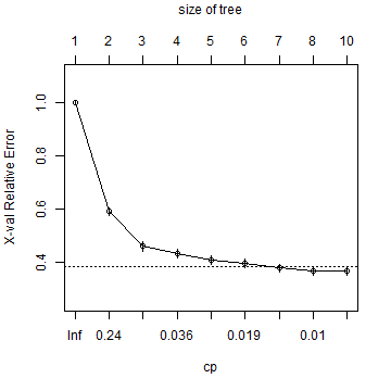
And here is the tree

plot(cart, uniform=TRUE, main="Regression Tree")
# text(cart, use.n=TRUE, all=TRUE, cex=.8)
text(cart, cex=.8, digits=1)

Question 1: Describe the conditions under which you have the highest probability of finding our beloved species?

Random Forest¶

CART gives us a nice result to look at that can be easily interpreted (as you just illustrated with your answer to Question 1). But the approach suffers from high variance (meaning that the model will be over-fit, it is different each time a somewhat different datasets are used). Random Forest does not have that problem as much. Above, with CART, we use regression, let’s do both regression and classification here. First classification.

library(randomForest)
## randomForest 4.6-14
## Type rfNews() to see new features/changes/bug fixes.
# create a factor to indicated that we want classification
fpa <- as.factor(dw[, 'pa'])

Now fit the RandomForest model

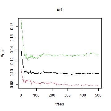
crf <- randomForest(dw[, 2:ncol(dw)], fpa)
crf
##
## Call:
##  randomForest(x = dw[, 2:ncol(dw)], y = fpa)
##                Type of random forest: classification
##                      Number of trees: 500
## No. of variables tried at each split: 4
##
##         OOB estimate of  error rate: 9.92%
## Confusion matrix:
##      0    1 class.error
## 0 1862  160  0.07912957
## 1  162 1062  0.13235294
plot(crf)

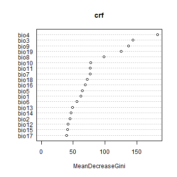
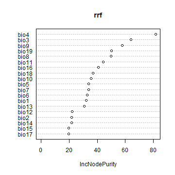
The variable importance plot shows which variables are most important in fitting the model. This is computing by randomizing each variable one by one and then computing the decline in model prediction.

varImpPlot(crf)

Now we use regression, rather than classification. First we tune a parameter.

trf <- tuneRF(dw[, 2:ncol(dw)], dw[, 'pa'])
## Warning in randomForest.default(x, y, mtry = mtryStart, ntree = ntreeTry, :
## The response has five or fewer unique values. Are you sure you want to do
## regression?
## mtry = 6  OOB error = 0.07223543
## Searching left ...
## Warning in randomForest.default(x, y, mtry = mtryCur, ntree = ntreeTry, :
## The response has five or fewer unique values. Are you sure you want to do
## regression?
## mtry = 3     OOB error = 0.07002109
## 0.03065438 0.05
## Searching right ...
## Warning in randomForest.default(x, y, mtry = mtryCur, ntree = ntreeTry, :
## The response has five or fewer unique values. Are you sure you want to do
## regression?
## mtry = 12    OOB error = 0.07146042
## 0.01072891 0.05

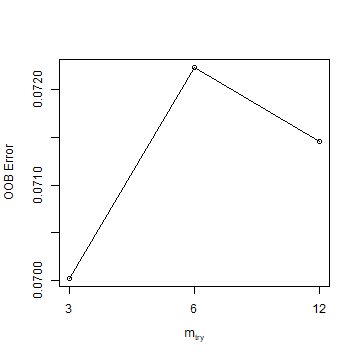
trf
##    mtry   OOBError
## 3     3 0.07002109
## 6     6 0.07223543
## 12   12 0.07146042
mt <- trf[which.min(trf[,2]), 1]
mt
## [1] 3

Question 2: What did tuneRF help us find? What does the values of mt represent?

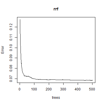
rrf <- randomForest(dw[, 2:ncol(d)], dw[, 'pa'], mtry=mt)
## Warning in randomForest.default(dw[, 2:ncol(d)], dw[, "pa"], mtry = mt):
## The response has five or fewer unique values. Are you sure you want to do
## regression?
rrf
##
## Call:
##  randomForest(x = dw[, 2:ncol(d)], y = dw[, "pa"], mtry = mt)
##                Type of random forest: regression
##                      Number of trees: 500
## No. of variables tried at each split: 3
##
##           Mean of squared residuals: 0.06842395
##                     % Var explained: 70.87
plot(rrf)

varImpPlot(rrf)

Predict¶

We can use the model to make predictions to any other place for which we have values for the predictor variables. Our climate data is global so we could find suitable places for bigfoot in Australia. At first I only want to predict to our study region, which I define as follows.

# Extent of the western points
ew <- extent(SpatialPoints(bf[bf[,1] <= -102, 1:2]))
ew
## class      : Extent
## xmin       : -156.75
## xmax       : -102.3881
## ymin       : 30.77722
## ymax       : 69.5

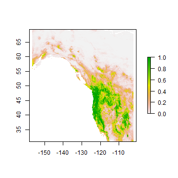
Regression¶

rp <- predict(wc, rrf, ext=ew)
plot(rp)

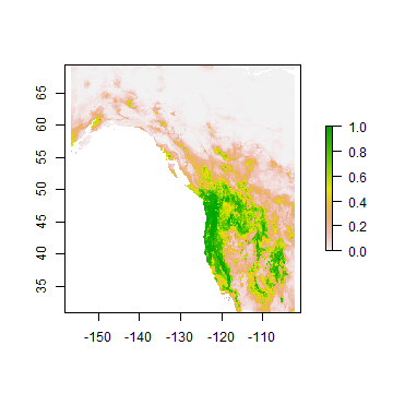
Note that the regression predictions are well-behaved, in the sense that they are between 0 and 1. However, they are continuous within that range, and if you wanted presence/absence, you would need a threshold. To get the optimal threshold, you would normally have a hold out data set, but here I used the training data for simplicity.

eva <- evaluate(dw[dw$pa==1, ], dw[dw$pa==0, ], rrf)
eva
## class          : ModelEvaluation
## n presences    : 1224
## n absences     : 2022
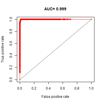
## AUC            : 0.9993911
## cor            : 0.964508
## max TPR+TNR at : 0.4982011

We can make a ROC plot

plot(eva, 'ROC')

Find a good threshold to determine presence/absence and plot the prediction.

tr <- threshold(eva)
tr
##                kappa spec_sens no_omission prevalence equal_sens_spec
## thresholds 0.4982011 0.4982011   0.3976191  0.3785858       0.5176767
##            sensitivity
## thresholds   0.7221367
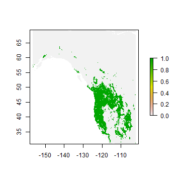
plot(rp > tr[1, 'spec_sens'])

Classification¶

We can also use the classification Random Forest model to make a prediction.

rc <- predict(wc, crf, ext=ew)
plot(rc)

You can also get probabilities for the classes

rc2 <- predict(wc, crf, ext=ew, type='prob', index=2)
plot(rc2)

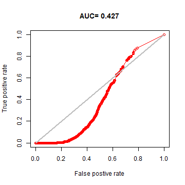
Extrapolation¶

Now, let’s see if our model is general enough to predict the distribution of the Eastern species.

de <- na.omit(de)
eva2 <- evaluate(de[de$pa==1, ], de[de$pa==0, ], rrf)
eva2
## class          : ModelEvaluation
## n presences    : 1866
## n absences     : 2978
## AUC            : 0.4271887
## cor            : -0.260545
## max TPR+TNR at : 3e-04
plot(eva2, 'ROC')

We can also look at it on a map.

eus <- extent(SpatialPoints(bf[, 1:2]))
eus
## class      : Extent
## xmin       : -156.75
## xmax       : -64.4627
## ymin       : 25.141
## ymax       : 69.5
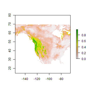
rcusa <- predict(wc, rrf, ext=eus)
plot(rcusa)
points(bf[,1:2], cex=.25)

Question 3: Why would it be that the model does not extrapolate well?

An important question in the biogeography of the western species is why it does not occur in Mexico. Or if it does, where would that be?

Let’s see.

mex <- getData('GADM', country='MEX', level=1)
pm <- predict(wc, rrf, ext=mex)
pm <- mask(pm, mex)
plot(pm)

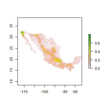
Question 4: Where in Mexico are you most likely to encounter western bigfoot?

We can also estimate range shifts due to climate change

fut <- getData('CMIP5', res=10, var='bio', rcp=85, model='AC', year=70)
names(fut)
##  [1] "ac85bi701"  "ac85bi702"  "ac85bi703"  "ac85bi704"  "ac85bi705"
##  [6] "ac85bi706"  "ac85bi707"  "ac85bi708"  "ac85bi709"  "ac85bi7010"
## [11] "ac85bi7011" "ac85bi7012" "ac85bi7013" "ac85bi7014" "ac85bi7015"
## [16] "ac85bi7016" "ac85bi7017" "ac85bi7018" "ac85bi7019"
names(wc)
##  [1] "bio1"  "bio2"  "bio3"  "bio4"  "bio5"  "bio6"  "bio7"  "bio8"  "bio9"
## [10] "bio10" "bio11" "bio12" "bio13" "bio14" "bio15" "bio16" "bio17" "bio18"
## [19] "bio19"
names(fut) <- names(wc)
futusa <- predict(fut, rrf, ext=eus, progress='window')
## Loading required namespace: tcltk
plot(futusa)

Question 5: Make a map to show where conditions are improving for western bigfoot, and where they are not. Is the species headed toward extinction?