Processing
Here we crop an image to get an exact area of interest, and then we compute the Normalized Difference Vegetation Index (NDVI).
Get the polygon boundary
library(terra)
## terra 1.9.21
library(geodata)
ken <- gadm(country="KEN", level=1, path=".")
pol <- ken[ken$NAME_1 == "Marsabit", ]
Change vector boundary coordinate reference system, so that it matches that of the MODIS data.
datadir <- file.path(dirname(tempdir()), "_modis")
mf <- file.path(datadir, "modis_qualmasked.tif")
rmask <- rast(mf)
prj <- crs(rmask)
prj
## [1] "PROJCRS[\"unnamed\",\n    BASEGEOGCRS[\"Unknown datum based upon the custom spheroid\",\n        DATUM[\"Not specified (based on custom spheroid)\",\n            ELLIPSOID[\"Custom spheroid\",6371007.181,0,\n                LENGTHUNIT[\"metre\",1,\n                    ID[\"EPSG\",9001]]]],\n        PRIMEM[\"Greenwich\",0,\n            ANGLEUNIT[\"degree\",0.0174532925199433,\n                ID[\"EPSG\",9122]]]],\n    CONVERSION[\"Sinusoidal\",\n        METHOD[\"Sinusoidal\"],\n        PARAMETER[\"Longitude of natural origin\",0,\n            ANGLEUNIT[\"degree\",0.0174532925199433],\n            ID[\"EPSG\",8802]],\n        PARAMETER[\"False easting\",0,\n            LENGTHUNIT[\"metre\",1],\n            ID[\"EPSG\",8806]],\n        PARAMETER[\"False northing\",0,\n            LENGTHUNIT[\"metre\",1],\n            ID[\"EPSG\",8807]]],\n    CS[Cartesian,2],\n        AXIS[\"easting\",east,\n            ORDER[1],\n            LENGTHUNIT[\"metre\",1,\n                ID[\"EPSG\",9001]]],\n        AXIS[\"northing\",north,\n            ORDER[2],\n            LENGTHUNIT[\"metre\",1,\n                ID[\"EPSG\",9001]]]]"
poly <- project(pol, prj)
Question: Why do not we change the coordinate system of the MODIS data?
Crop the image using the transformed vector boundaries.
rcrop <- crop(rmask, poly)
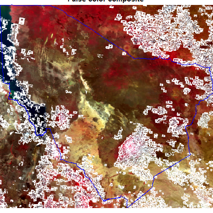
Plot cropped MODIS and add the boundary. We use plotRGB to make a false color composite (near-infrared, red, green)
plotRGB(rcrop, r = 2, g = 1, b = 4,  main = "False color composite", stretch = "lin" )
lines(poly, col="blue")
NDVI
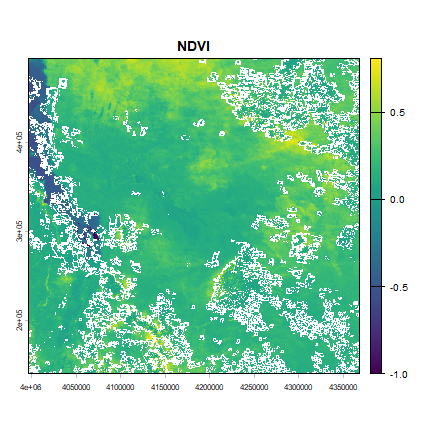
We have so far masked out bad quality pixels and clipped the image to area of interest extents. Let us now use the processed image to compute an index measure. The Normalized Difference Vegetation Index (NDVI) is a common measure of greenness. It is computed as follows
We expect the reflectance to be between 0 (very dark areas) and 1 (very bright areas). Due to various reasons, there may values slightly outside this rnage. First clamp values of the image between 0 and 1.
r <- clamp(rcrop, 0, 1)
ndvi <- (r[[2]] - r[[1]]) /(r[[2]] + r[[1]])
plot(ndvi, main="NDVI")
Exercise Write a function to compute NDVI type two-band spectral
indices and compute NDVI using the function.