Image exploration
Introduction
Now that we have successfully downloaded one MODIS tile, we can use
terra package to explore and visualize it. Please note that MODIS
tiles are distributed in HDF format that may include sub-datasets. The
sub-dataset and processing steps might be different for various MODIS
collections (e.g. daily scenes, vegetation indices).
Now that we have download some MODIS data, we can explore and visualize it.
First create a SpatRaster object from the file created on the previous page.
datadir <- file.path(dirname(tempdir()), "_modis")
mf <- file.path(datadir, "MOD09A1.A2009361.h21v08.061.2021149144347.hdf")
library(terra)
r <- rast(mf[1])
r
## class       : SpatRaster
## size        : 2400, 2400, 13  (nrow, ncol, nlyr)
## resolution  : 463.3127, 463.3127  (x, y)
## extent      : 3335852, 4447802, 0, 1111951  (xmin, xmax, ymin, ymax)
## coord. ref. : +proj=sinu +lon_0=0 +x_0=0 +y_0=0 +R=6371007.181 +units=m +no_defs
## sources     : MOD09A1.A2009361.h21v08.061.2021149144347.hdf:MOD_Grid_500m_Surface_Reflectance:sur_refl_b01
##               MOD09A1.A2009361.h21v08.061.2021149144347.hdf:MOD_Grid_500m_Surface_Reflectance:sur_refl_b02
##               MOD09A1.A2009361.h21v08.061.2021149144347.hdf:MOD_Grid_500m_Surface_Reflectance:sur_refl_b03
##               ... and 10 more sources
## names       : sur_refl_b01, sur_refl_b02, sur_refl_b03, sur_refl_b04, sur_refl_b05, sur_refl_b06, ...
Exercise: Find out at least 5 properties (path, row, date of collection etc) of the MODIS data from the information embedded in the filename.
Image properties
The code below illustrates how you can load HDF files and access image properties of a SpatRaster object.
The coordinate reference system (CRS)
crs(r)
## [1] "PROJCRS[\"unnamed\",\n    BASEGEOGCRS[\"Unknown datum based upon the custom spheroid\",\n        DATUM[\"Not specified (based on custom spheroid)\",\n            ELLIPSOID[\"Custom spheroid\",6371007.181,0,\n                LENGTHUNIT[\"metre\",1,\n                    ID[\"EPSG\",9001]]]],\n        PRIMEM[\"Greenwich\",0,\n            ANGLEUNIT[\"degree\",0.0174532925199433,\n                ID[\"EPSG\",9122]]]],\n    CONVERSION[\"Sinusoidal\",\n        METHOD[\"Sinusoidal\"],\n        PARAMETER[\"Longitude of natural origin\",0,\n            ANGLEUNIT[\"degree\",0.0174532925199433],\n            ID[\"EPSG\",8802]],\n        PARAMETER[\"False easting\",0,\n            LENGTHUNIT[\"metre\",1],\n            ID[\"EPSG\",8806]],\n        PARAMETER[\"False northing\",0,\n            LENGTHUNIT[\"metre\",1],\n            ID[\"EPSG\",8807]]],\n    CS[Cartesian,2],\n        AXIS[\"(E)\",east,\n            ORDER[1],\n            LENGTHUNIT[\"Meter\",1]],\n        AXIS[\"(N)\",north,\n            ORDER[2],\n            LENGTHUNIT[\"Meter\",1]]]"
And the number of cells, rows, columns
dim(r)
## [1] 2400 2400   13
nrow(r)
## [1] 2400
ncol(r)
## [1] 2400
# Number of layers (bands)
nlyr(r)
## [1] 13
ncell(r)
## [1] 5760000
The spatial resolution is about 500 m
res(r)
## [1] 463.3127 463.3127
The layernames tell us what “bands” we have
names(r)
##  [1] "sur_refl_b01"         "sur_refl_b02"         "sur_refl_b03"
##  [4] "sur_refl_b04"         "sur_refl_b05"         "sur_refl_b06"
##  [7] "sur_refl_b07"         "sur_refl_qc_500m"     "sur_refl_szen"
## [10] "sur_refl_vzen"        "sur_refl_raz"         "sur_refl_state_500m"
## [13] "sur_refl_day_of_year"
Plot
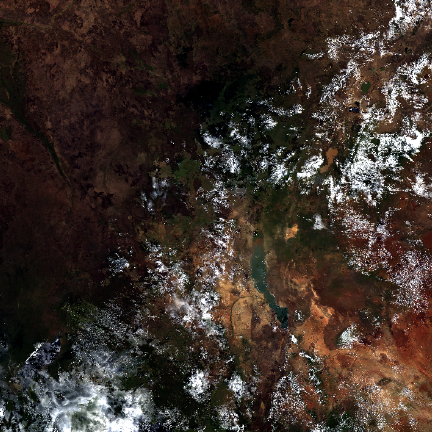
Now let’s make some simple plots to see if things look reasonable.
# Create an image RGB composite plot
plotRGB(r, r = 1, g = 4, b = 3)

# Disappointing? apply some stretching; see `?plotRGB` for more options
plotRGB(r, r = 1, g = 4, b = 3, stretch="lin")
Exercise: Create False Color Composite plot using the same data. Hint:
try plotRGB and specify the bands you need.
Exercise: Save the plots to graphics files. Hint: have a look at
?png.