Supervised Classification
Here we explore supervised classification for a simple land use land cover (LULC) mapping task. Various supervised classification algorithms exist, and the choice of algorithm can affect the results. Here we explore two related algorithms (CART and RandomForest).
In supervised classification, we have prior knowledge about some of the land-cover types through, for example, fieldwork, reference spatial data or interpretation of high resolution imagery (such as available on Google maps). Specific sites in the study area that represent homogeneous examples of these known land-cover types are identified. These areas are commonly referred to as training sites because the spectral properties of these sites are used to train the classification algorithm.
The following examples uses a Classification and Regression Trees (CART) classifier (Breiman et al. 1984) (further reading to predict land use land cover classes in the study area.
We will take the following steps:
Create sample sites used for classification
Extract cell values from Landsat data for the sample sites
Train the classifier using training samples
Classify the Landsat data using the trained model
Evaluate the accuracy of the model
Landsat data to classify
Here is our Landsat data.
library(terra)
## terra 1.9.21
# We read the 6 bands from the Landsat image we previously used
raslist <- paste0('data/rs/LC08_044034_20170614_B', 2:7, ".tif")
landsat <- rast(raslist)
names(landsat) <- c('blue', 'green', 'red', 'NIR', 'SWIR1', 'SWIR2')
Reference data
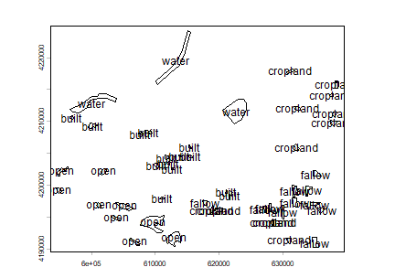
Training and/or validation data can come from a variety of sources. In this example, we use some training polygons we have already collected from other sources. We have already used this for making the spectral plots.There are 5 distinct classes – built,cropland,fallow,open and, water and we hope to find the pixels under this categroies based on our knowledge of training sites.
# load polygons with land use land cover information
samp <- readRDS("data/rs/lcsamples.rds")
# check the distribution of the polygons
plot(samp)
text(samp, samp$class)
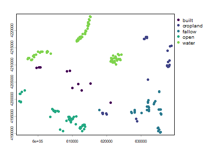
Next we generate random points within each polygons.
set.seed(1)
# generate point samples from the polygons
ptsamp <- spatSample(samp, 200, method="random")
plot(ptsamp, "class")
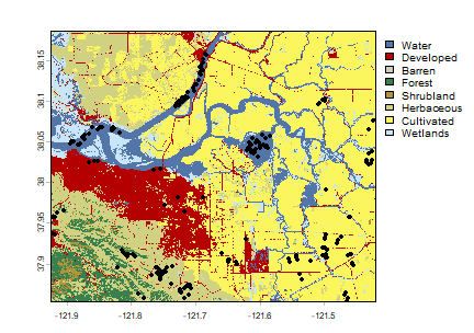
Alternatively, we can generate the training and validation sample sites using a reference land use land cover data. For example, the National Land Cover Database 2011 (NLCD 2011) is a land cover product for the United States. NLCD is a 30-m Landsat-based land cover database spanning 4 epochs (1992, 2001, 2006 and 2011). NLCD 2011 is based primarily on a decision-tree classification of circa 2011 Landsat data.
Detailes of the class mapped in NCLD 2011 can be found here (here)[https://www.mrlc.gov/nlcd11_leg.php]. It has two pairs of class values and names that correspond to the levels of land use and land cover classification system. These levels usually represent the level of complexity, level I being the simplest with broad land use land cover categories. Read this report by Anderson et al to learn more about this land use and land cover classification system.
nlcd <- rast('data/rs/nlcd-L1.tif')
names(nlcd) <- c("nlcd2001", "nlcd2011")
nlcd2011 <- nlcd[[2]]
# assign class names as categories (levels)
nlcdclass <- c("Water", "Developed", "Barren", "Forest", "Shrubland", "Herbaceous", "Cultivated", "Wetlands")
classdf <- data.frame(value = c(1,2,3,4,5,7,8,9), names = nlcdclass)
levels(nlcd2011) <- classdf
# colors (as hexidecimal codes)
classcolor <- c("#5475A8", "#B50000", "#D2CDC0", "#38814E", "#AF963C", "#D1D182", "#FBF65D", "#C8E6F8")
# plot the locations on top of the original nlcd raster
plot(nlcd2011, col=classcolor)
ptlonlat <- project(ptsamp, crs(nlcd2011))
points(ptlonlat)
Generate sample sites from the NLCD SpatRaster
# Sampling
samp2011 <- spatSample(nlcd2011, size = 200, method="regular")
# Number of samples in each class
table(samp2011[,1])
##
##      Water  Developed     Barren     Forest  Shrubland Herbaceous Cultivated
##         19         29          1          6          3         35        107
##   Wetlands
##         16
Extract reflectance values for the training sites
Once we have the training sites, we can extract the cell values from
each layer in landsat. These values will be the predictor variables
and “class” from ptsamp will be the response variable.
# extract the reflectance values for the locations
df <- extract(landsat, ptsamp, ID=FALSE)
# Quick check for the extracted values
head(df)
##         blue      green        red        NIR       SWIR1       SWIR2
## 1 0.09797934 0.08290726 0.05811966 0.01958285 0.006245691 0.003816809
## 2 0.11986095 0.09904197 0.07978442 0.05723051 0.040965684 0.033939276
## 3 0.12838373 0.13727517 0.18810819 0.31336907 0.315103978 0.180648044
## 4 0.15295446 0.18123358 0.25232175 0.40375817 0.401546150 0.237791821
## 5 0.13992092 0.14987499 0.19207680 0.28279120 0.356763631 0.232044920
## 6 0.12341753 0.10114556 0.08288557 0.06377982 0.046972826 0.038883783
# combine lulc class information with extracted values
sampdata <- data.frame(class = ptsamp$class, df)
We often find classnames are provided as string labels (e.g. water, crop, vegetation) that need to be ‘relabelled’ to integer or factors if only string labels are supplied before using them as response variable in the classification. There are several approaches that could be used to convert these classes to integer codes. We can make a function that will reclassify the character strings representing land cover classes into integers based on the existing factor levels.
Train the classifier
Now we will train the classification algorithm using sampdata
dataset.
library(rpart)
# Train the model
cartmodel <- rpart(as.factor(class)~., data = sampdata, method = 'class', minsplit = 5)
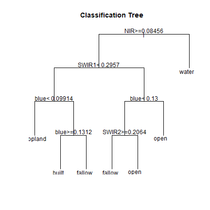
One of the primary reasons behind choosing cart model is to have a
closer look at the classification model. Unlike other models, cart
provides very simple way of inspecting and plotting the model structure.
# print trained model
print(cartmodel)
## n= 200
##
## node), split, n, loss, yval, (yprob)
##       * denotes terminal node
##
##  1) root 200 122 water (0.055 0.12 0.19 0.24 0.39)
##    2) NIR>=0.08455543 122  73 open (0.09 0.2 0.31 0.4 0)
##      4) SWIR1< 0.2957055 70  35 fallow (0.14 0.34 0.5 0.014 0)
##        8) blue< 0.09913956 24   0 cropland (0 1 0 0 0) *
##        9) blue>=0.09913956 46  11 fallow (0.22 0 0.76 0.022 0)
##         18) blue>=0.1312463 10   0 built (1 0 0 0 0) *
##         19) blue< 0.1312463 36   1 fallow (0 0 0.97 0.028 0) *
##      5) SWIR1>=0.2957055 52   4 open (0.019 0 0.058 0.92 0)
##       10) blue< 0.1299668 13   3 open (0 0 0.23 0.77 0)
##         20) SWIR2>=0.2063899 3   0 fallow (0 0 1 0 0) *
##         21) SWIR2< 0.2063899 10   0 open (0 0 0 1 0) *
##       11) blue>=0.1299668 39   1 open (0.026 0 0 0.97 0) *
##    3) NIR< 0.08455543 78   0 water (0 0 0 0 1) *
# Plot the trained classification tree
plot(cartmodel, uniform=TRUE, main="Classification Tree")
text(cartmodel, cex = 1)
See ?rpart.control to set different parameters for building the
model.
You can print/plot more about the cartmodel created in the previous
example. E.g. you can use plotcp(cartmodel) to learn about the
cost-complexity (cp argument in rpart).
Classify
Now that we have our trained classification model (cartmodel), we
can use it to make predictions, that is, to classify all cells in the
landsat5 SpatRaster.
Important The layer names in the SpatRaster should exactly match those that were used to train the model. This will be the case if the same SpatRaster object was used (via extract) to obtain the values to fit the model. Otherwise you need to specify the matching names.
classified <- predict(landsat, cartmodel, na.rm = TRUE)
classified
## class       : SpatRaster
## size        : 1245, 1497, 5  (nrow, ncol, nlyr)
## resolution  : 30, 30  (x, y)
## extent      : 594090, 639000, 4190190, 4227540  (xmin, xmax, ymin, ymax)
## coord. ref. : WGS 84 / UTM zone 10N (EPSG:32610)
## source(s)   : memory
## names       : built, cropland, fallow, open, water
## min values  :     0,        0,      0,    0,     0
## max values  :     1,        1,      1,    1,     1
plot(classified)
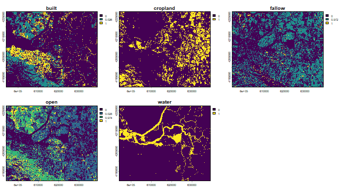
Observe that there are 5 layers in the classified object, each of
the layer representing the probability of a particular LULC class.
Below, we make a SpatRaster that shows, for each grid cell, the LULC
class with the highest probability.
lulc <- which.max(classified)
lulc
## class       : SpatRaster
## size        : 1245, 1497, 1  (nrow, ncol, nlyr)
## resolution  : 30, 30  (x, y)
## extent      : 594090, 639000, 4190190, 4227540  (xmin, xmax, ymin, ymax)
## coord. ref. : WGS 84 / UTM zone 10N (EPSG:32610)
## source(s)   : memory
## name        : which.max
## min value   :         1
## max value   :         5
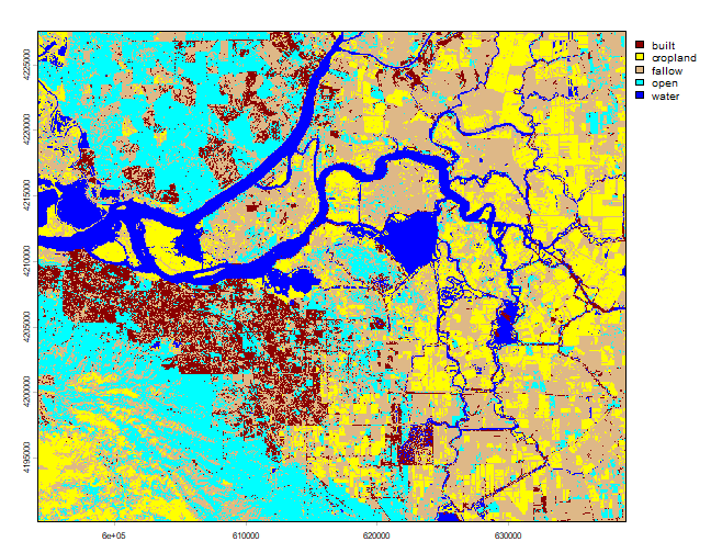
To make a nice map, we make the raster categorical, using levels<-;
and we provide custom colors.
cls <- c("built","cropland","fallow","open","water")
df <- data.frame(id = 1:5, class=cls)
levels(lulc) <- df
lulc
## class       : SpatRaster
## size        : 1245, 1497, 1  (nrow, ncol, nlyr)
## resolution  : 30, 30  (x, y)
## extent      : 594090, 639000, 4190190, 4227540  (xmin, xmax, ymin, ymax)
## coord. ref. : WGS 84 / UTM zone 10N (EPSG:32610)
## source(s)   : memory
## name        : class
## min value   :     1
## max value   :     5
mycolor <- c("darkred", "yellow", "burlywood", "cyan", "blue")
plot(lulc, col=mycolor)
If you are not satisfied with the results, you can select more samples and use additional predictor variables to see if you can improve the classification. The choice of classifier (algorithm) also plays an important role. Next we show how to test the performance the classification model.
Model evaluation
This section discusses how to assess the accuracy of the model to get an idea of how accurate the classified map might be. Two widely used measures in remote sensing are “overall accuracy” and “kappa”. You can perform the accuracy assessment using the independent samples.
To evaluate any model, you can use k-fold cross-validation (you can also
do single-fold). In this technique the data used to fit the model is
split into k groups (typically 5 groups). In turn, one of the groups
will be used for model testing, while the rest of the data is used for
model training (fitting).
set.seed(99)
# number of folds
k <- 5
j <- sample(rep(1:k, each = round(nrow(sampdata))/k))
table(j)
## j
##  1  2  3  4  5
## 40 40 40 40 40
Now we train and test the model five times, each time computing the predictions and storing that with the actual values in a list. Later we use the list to compute the final accuarcy.
x <- list()
for (k in 1:5) {
    train <- sampdata[j!= k, ]
    test <- sampdata[j == k, ]
    cart <- rpart(as.factor(class)~., data=train, method = 'class',
                  minsplit = 5)
    pclass <- predict(cart, test, na.rm = TRUE)
    # assign class to maximum probablity
    pc <- apply(pclass, 1, which.max)
    # use labels instead of numbers
    pc <- colnames(pclass)[pc]
    # create a data.frame using the reference and prediction
    x[[k]] <- cbind(test$class, pc)
}
Now combine the five list elements into a single data.frame, using
do.call and compute a confusion matrix.
y <- do.call(rbind, x)
y <- data.frame(y)
colnames(y) <- c('observed', 'predicted')
# confusion matrix
conmat <- table(y)
print(conmat)
##           predicted
## observed   built cropland fallow open water
##   built        8        0      1    2     0
##   cropland     0       24      0    0     0
##   fallow       2        0     33    3     0
##   open         0        0      2   47     0
##   water        0        0      0    0    78
Question 1:Comment on the miss-classification between different classes.
Question 2:Can you think of ways to to improve the accuracy.
Compute the overall accuracy and the “kappa” statistic.
Overall accuracy:
# number of total cases/samples
n <- sum(conmat)
n
## [1] 200
# number of correctly classified cases per class
diag <- diag(conmat)
# Overall Accuracy
OA <- sum(diag) / n
OA
## [1] 0.95
Kappa:
# observed (true) cases per class
rowsums <- apply(conmat, 1, sum)
p <- rowsums / n
# predicted cases per class
colsums <- apply(conmat, 2, sum)
q <- colsums / n
expAccuracy <- sum(p*q)
kappa <- (OA - expAccuracy) / (1 - expAccuracy)
kappa
## [1] 0.9317732
Producer and user accuracy
# Producer accuracy
PA <- diag / colsums
# User accuracy
UA <- diag / rowsums
outAcc <- data.frame(producerAccuracy = PA, userAccuracy = UA)
outAcc
##          producerAccuracy userAccuracy
## built           0.8000000    0.7272727
## cropland        1.0000000    1.0000000
## fallow          0.9166667    0.8684211
## open            0.9038462    0.9591837
## water           1.0000000    1.0000000
Question 3:Perform the classification using Random Forest classifiers from the ``randomForest`` package
Question 4:Plot the results of rpart and Random Forest classifier side-by-side.
Question 5 (optional):Repeat the steps for other years using Random
Forest. For example you can use the cloud-free composite image
data/centralvalley-2001LE7.tif. This data is collected by the
Landsat 7 platform. You
can use the National Land Cover Database 2001 (NLCD
2001) subset of the California
Central Valley for generating training sites.
Question 6 (optional):We have trained the classifiers using unequal samples for each class. Investigate the effect of sample size on classification. Repeat the steps with different subsets, e.g. a sample size of 100, 50, 25 per class, and compare the results. Use the same holdout samples for model evaluation.