Exploration
In this chapter we describe how to explore satellite remote sensing data with R. We also show how to use them to make maps.
We will primarily use a spatial subset of a Landsat 8 scene collected on June 14, 2017. The subset covers the area between Concord and Stockton, in California, USA.
All Landsat scenes have a unique product ID and metadata. You can find the information on Landsat sensor, satellite, location on Earth (WRS path, WRS row) and acquisition date from the product ID. For example, the product identifier of the data we will use is ‘LC08_044034_20170614’. Based on this guide, you can see that the Sensor-Satellite is OLI/TIRS combined Landsat 8, WRS Path 44, WRS Row 34 and collected on June 14, 2017. Landsat scenes are most commonly delivered as separate files for each band, combined into a single zip file.
We will start by exploring and visualizing the data (See the instructions in Chapter 1 for data downloading instructions if you have not already done so).
Image properties
Create SpatRaster objects for single Landsat layers (bands)
library(terra)
## terra 1.9.21
# Blue
b2 <- rast('data/rs/LC08_044034_20170614_B2.tif')
# Green
b3 <- rast('data/rs/LC08_044034_20170614_B3.tif')
# Red
b4 <- rast('data/rs/LC08_044034_20170614_B4.tif')
# Near Infrared (NIR)
b5 <- rast('data/rs/LC08_044034_20170614_B5.tif')
Print the variables to check. E.g.
b2
## class       : SpatRaster
## size        : 1245, 1497, 1  (nrow, ncol, nlyr)
## resolution  : 30, 30  (x, y)
## extent      : 594090, 639000, 4190190, 4227540  (xmin, xmax, ymin, ymax)
## coord. ref. : WGS 84 / UTM zone 10N (EPSG:32610)
## source      : LC08_044034_20170614_B2.tif
## name        : LC08_044034_20170614_B2
## min value   :                 0.07484
## max value   :                0.717756
You can see the spatial resolution, extent, number of layers, coordinate reference system and more.
Image information and statistics
The below shows how you can access various properties from a SpatRaster object.
# coordinate reference system (CRS)
crs(b2)
## [1] "PROJCRS[\"WGS 84 / UTM zone 10N\",\n    BASEGEOGCRS[\"WGS 84\",\n        DATUM[\"World Geodetic System 1984\",\n            ELLIPSOID[\"WGS 84\",6378137,298.257223563,\n                LENGTHUNIT[\"metre\",1]]],\n        PRIMEM[\"Greenwich\",0,\n            ANGLEUNIT[\"degree\",0.0174532925199433]],\n        ID[\"EPSG\",4326]],\n    CONVERSION[\"UTM zone 10N\",\n        METHOD[\"Transverse Mercator\",\n            ID[\"EPSG\",9807]],\n        PARAMETER[\"Latitude of natural origin\",0,\n            ANGLEUNIT[\"degree\",0.0174532925199433],\n            ID[\"EPSG\",8801]],\n        PARAMETER[\"Longitude of natural origin\",-123,\n            ANGLEUNIT[\"degree\",0.0174532925199433],\n            ID[\"EPSG\",8802]],\n        PARAMETER[\"Scale factor at natural origin\",0.9996,\n            SCALEUNIT[\"unity\",1],\n            ID[\"EPSG\",8805]],\n        PARAMETER[\"False easting\",500000,\n            LENGTHUNIT[\"metre\",1],\n            ID[\"EPSG\",8806]],\n        PARAMETER[\"False northing\",0,\n            LENGTHUNIT[\"metre\",1],\n            ID[\"EPSG\",8807]]],\n    CS[Cartesian,2],\n        AXIS[\"(E)\",east,\n            ORDER[1],\n            LENGTHUNIT[\"metre\",1]],\n        AXIS[\"(N)\",north,\n            ORDER[2],\n            LENGTHUNIT[\"metre\",1]],\n    USAGE[\n        SCOPE[\"Navigation and medium accuracy spatial referencing.\"],\n        AREA[\"Between 126°W and 120°W, northern hemisphere between equator and 84°N, onshore and offshore. Canada - British Columbia (BC); Northwest Territories (NWT); Nunavut; Yukon. United States (USA) - Alaska (AK).\"],\n        BBOX[0,-126,84,-120]],\n    ID[\"EPSG\",32610]]"
# Number of cells, rows, columns
ncell(b2)
## [1] 1863765
dim(b2)
## [1] 1245 1497    1
# spatial resolution
res(b2)
## [1] 30 30
# Number of layers (bands in remote sensing jargon)
nlyr(b2)
## [1] 1
# Do the bands have the same extent, number of rows and columns, projection, resolution, and origin
compareGeom(b2,b3)
## [1] TRUE
You can create a SpatRaster with multiple layers from the existing SpatRaster (single layer) objects.
s <- c(b5, b4, b3)
# Check the properties of the multi-band image
s
## class       : SpatRaster
## size        : 1245, 1497, 3  (nrow, ncol, nlyr)
## resolution  : 30, 30  (x, y)
## extent      : 594090, 639000, 4190190, 4227540  (xmin, xmax, ymin, ymax)
## coord. ref. : WGS 84 / UTM zone 10N (EPSG:32610)
## sources     : LC08_044034_20170614_B5.tif
##               LC08_044034_20170614_B4.tif
##               LC08_044034_20170614_B3.tif
## names       : LC08_04403~0170614_B5, LC08_04403~0170614_B4, LC08_04403~0170614_B3
## min values  :              0.000846,              0.020841,              0.042592
## max values  :              1.012432,              0.786177,               0.69247
You can also create the multi-layer SpatRaster using the filenames.
# first create a list of raster layers to use
filenames <- paste0('data/rs/LC08_044034_20170614_B', 1:11, ".tif")
filenames
##  [1] "data/rs/LC08_044034_20170614_B1.tif"
##  [2] "data/rs/LC08_044034_20170614_B2.tif"
##  [3] "data/rs/LC08_044034_20170614_B3.tif"
##  [4] "data/rs/LC08_044034_20170614_B4.tif"
##  [5] "data/rs/LC08_044034_20170614_B5.tif"
##  [6] "data/rs/LC08_044034_20170614_B6.tif"
##  [7] "data/rs/LC08_044034_20170614_B7.tif"
##  [8] "data/rs/LC08_044034_20170614_B8.tif"
##  [9] "data/rs/LC08_044034_20170614_B9.tif"
## [10] "data/rs/LC08_044034_20170614_B10.tif"
## [11] "data/rs/LC08_044034_20170614_B11.tif"
landsat <- rast(filenames)
landsat
## class       : SpatRaster
## size        : 1245, 1497, 11  (nrow, ncol, nlyr)
## resolution  : 30, 30  (x, y)
## extent      : 594090, 639000, 4190190, 4227540  (xmin, xmax, ymin, ymax)
## coord. ref. : WGS 84 / UTM zone 10N (EPSG:32610)
## sources     : LC08_044034_20170614_B1.tif
##               LC08_044034_20170614_B2.tif
##               LC08_044034_20170614_B3.tif
##               ... and 8 more sources
## names       : LC08_~14_B1, LC08_~14_B2, LC08_~14_B3, LC08_~14_B4, LC08_~14_B5, LC08_~14_B6, ...
## min values  :    0.096418,     0.07484,    0.042592,    0.020841,    0.000846,   -0.007872, ...
## max values  :    0.734628,    0.717756,     0.69247,    0.786177,    1.012432,    1.043205, ...
Above we created a SpatRaster with 11 layers. The layers represent reflection intensity in the following wavelengths: Ultra Blue, Blue, Green, Red, Near Infrared (NIR), Shortwave Infrared (SWIR) 1, Shortwave Infrared (SWIR) 2, Panchromatic, Cirrus, Thermal Infrared (TIRS) 1, Thermal Infrared (TIRS) 2.
Single band and composite maps
You can plot individual layers of a multi-spectral image.
par(mfrow = c(2,2))
plot(b2, main = "Blue", col = gray(0:100 / 100))
plot(b3, main = "Green", col = gray(0:100 / 100))
plot(b4, main = "Red", col = gray(0:100 / 100))
plot(b5, main = "NIR", col = gray(0:100 / 100))
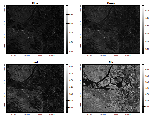
The legends of the maps created above can range between 0 and 1. Notice the difference in shading and range of legends between the different bands. This is because different surface features reflect the incident solar radiation differently. Each layer represent how much incident solar radiation is reflected for a particular wavelength range. For example, vegetation reflects more energy in NIR than other wavelengths and thus appears brighter. In contrast, water absorbs most of the energy in the NIR wavelength and it appears dark.
We do not gain that much information from these grey-scale plots; they are often combined into a “composite” to create more interesting plots. You can learn more about color composites in remote sensing here and also in the section below.
To make a “true (or natural) color” image, that is, something that looks
like a normal photograph (vegetation in green, water blue etc), we need
bands in the red, green and blue regions. For this Landsat image, band 4
(red), 3 (green), and 2 (blue) can be used. With plotRGB we can
combine them into a single composite image. Note that use of
strecth = "lin" (otherwise the image will be pitch-dark).
landsatRGB <- c(b4, b3, b2)
plotRGB(landsatRGB, stretch = "lin")
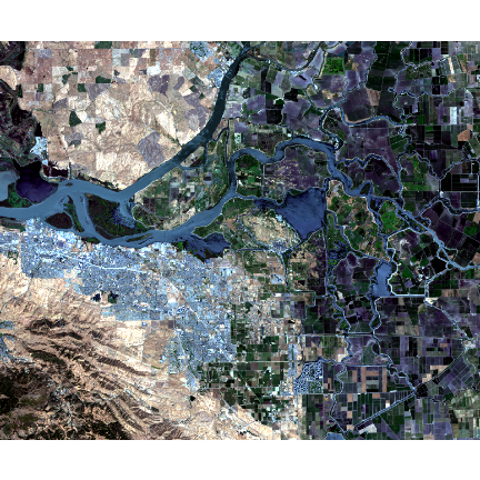
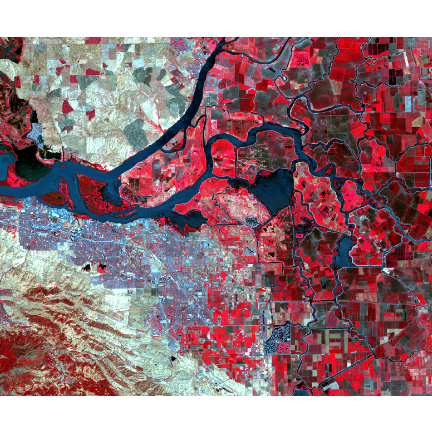
The true-color composite reveals much more about the landscape than the earlier gray images. Another popular image visualization method in remote sensing is known “false color” image in which NIR, red, and green bands are combined. This representation is popular as it makes it easy to see the vegetation (in red).
landsatFCC <- c(b5, b4, b3)
plotRGB(landsatFCC, stretch="lin")
Question 1: Now use the plotRGB function with the multi-band (11 layers) ``landsat`` SpatRaster to create a true and false color composite (hint remember the position of the bands).
Subset and rename bands
You can select specific layers (bands) using subset function, or via
indexing.
# select first 3 bands only
landsatsub1 <- subset(landsat, 1:3)
# same
landsatsub2 <- landsat[[1:3]]
# Number of bands in the original and new data
nlyr(landsat)
## [1] 11
nlyr(landsatsub1)
## [1] 3
nlyr(landsatsub2)
## [1] 3
We won’t use the last four bands in landsat. You can remove those by
selecting the ones we want.
landsat <- subset(landsat, 1:7)
For clarity, it is useful to set the names of the bands. (source)[https://www.usgs.gov/faqs/what-are-band-designations-landsat-satellites?qt-news_science_products=0#qt-news_science_products]
names(landsat)
## [1] "LC08_044034_20170614_B1" "LC08_044034_20170614_B2"
## [3] "LC08_044034_20170614_B3" "LC08_044034_20170614_B4"
## [5] "LC08_044034_20170614_B5" "LC08_044034_20170614_B6"
## [7] "LC08_044034_20170614_B7"
names(landsat) <- c('ultra-blue', 'blue', 'green', 'red', 'NIR', 'SWIR1', 'SWIR2')
names(landsat)
## [1] "ultra-blue" "blue"       "green"      "red"        "NIR"
## [6] "SWIR1"      "SWIR2"
Spatial subset or crop
Spatial subsetting can be used to limit analysis to a geographic subset
of the image. Spatial subsets can be created with the crop function,
using a SpatExtent object, or another spatial object from which an
Extent can be extracted.
ext(landsat)
## SpatExtent : 594090, 639000, 4190190, 4227540 (xmin, xmax, ymin, ymax)
e <- ext(624387, 635752, 4200047, 4210939)
# crop landsat by the extent
landsatcrop <- crop(landsat, e)
Question 2: Use the ``landsatcrop`` image to plot a true and false color composite
Saving results to disk
At this stage we may want to save the raster to disk with
writeRaster. Multiple file types are supported. We will use the
commonly used GeoTiff format.
writeRaster(landsatcrop, filename="cropped-landsat.tif", overwrite=TRUE)
Note: Check for package documentation (help(writeRaster)) for
additional helpful arguments that can be added.
Relation between bands
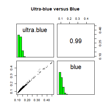
A scatterplot matrix can be helpful in exploring relationships between
raster layers. This can be done with the pairs function.
A plot of reflection in the ultra-blue wavelength against reflection in the blue wavelength.
pairs(landsatcrop[[1:2]], main = "Ultra-blue versus Blue")
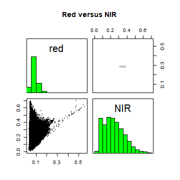
A plot of reflection in the red wavelength against reflection in the NIR wavelength.
pairs(landsatcrop[[4:5]], main = "Red versus NIR")
The first plot reveals high correlations between the blue wavelength regions. Because of the high correlation, we can just use one of the blue bands without losing much information.
This distribution of points in second plot (between NIR and red) is unique due to its triangular shape. Vegetation reflects very highly in the NIR range than red and creates the upper corner close to NIR (y) axis. Water absorbs energy from all the bands and occupies the location close to origin. The furthest corner is created due to highly reflecting surface features like bright soil or concrete (see Baret et al)[http://www.ipgp.fr/~jacquemoud/publications/baret1993a.pdf].
Extract cell values
Often we want to get the values of raster cells (pixels in remote
sensing jargon) for specific geographic locations or area. The
extract function is used to get raster values at the locations of
other spatial data. You can use points, lines, polygons or an Extent
(rectangle) object. You can also use cell numbers to extract values.
When using points, extract returns the values of a SpatRaster
object for the cells in which a set of points fall.
# load the polygons with land use land cover information
samp <- readRDS('data/rs/lcsamples.rds')
# generate 50 point samples from the polygons
set.seed(555)
ptsamp <- spatSample(samp, 50, 'regular')
# We use the x-y coordinates to extract the spectral values for the locations
df <- extract(landsat, ptsamp)
# To see some of the reflectance values
head(df)
##   ID ultra-blue       blue      green        red        NIR      SWIR1
## 1  1  0.1154152 0.09286134 0.08362291 0.05464983 0.43908536 0.16941448
## 2  2  0.1109912 0.08893609 0.08464217 0.05553897 0.38280904 0.09902029
## 3  3  0.1083455 0.08470724 0.07037250 0.04621380 0.33631334 0.16342902
## 4  4  0.1132900 0.09097461 0.08505422 0.05432453 0.45357192 0.20305014
## 5  5  0.1414823 0.12404644 0.10318408 0.08483735 0.06360633 0.04842582
## 6  6  0.1240898 0.10487562 0.07991453 0.05924735 0.03840668 0.01986478
##        SWIR2
## 1 0.08999872
## 2 0.04517285
## 3 0.07896033
## 4 0.08722286
## 5 0.03894885
## 6 0.01570098
Spectral profiles
A plot of the spectrum (all bands) for pixels representing a certain
earth surface features (e.g. water) is known as a spectral profile. Such
profiles demonstrate the differences in spectral properties of various
earth surface features and constitute the basis for image analysis.
Spectral values can be extracted from any multispectral data set using
extract function. In the above example, we extracted values of
Landsat data for the samples. These samples include: cropland, water,
fallow, built and open. First we compute the mean reflectance values for
each class and each band.
ms <- aggregate(df[,-1], list(ptsamp$class), mean)
# instead of the first column, we use row names
rownames(ms) <- ms[,1]
ms <- ms[,-1]
ms
##          ultra-blue       blue      green        red        NIR     SWIR1
## built     0.1786493 0.16950844 0.17206383 0.18493112 0.22927266 0.2335666
## cropland  0.1120105 0.08936982 0.08092295 0.05268178 0.40294491 0.1587285
## fallow    0.1304385 0.11181529 0.09206436 0.09047041 0.12907769 0.2044923
## open      0.1390433 0.13788239 0.15237471 0.20631468 0.34316624 0.3646445
## water     0.1327735 0.11559101 0.09775448 0.07715008 0.04756178 0.0319213
##               SWIR2
## built    0.19642493
## cropland 0.07533869
## fallow   0.19113344
## open     0.21842583
## water    0.02590160
Now we plot the mean spectra of these features.
# Create a vector of color for the land cover classes for use in plotting
mycolor <- c('darkred', 'yellow', 'burlywood', 'cyan', 'blue')
#transform ms from a data.frame to a matrix
ms <- as.matrix(ms)
# First create an empty plot
plot(0, ylim=c(0,0.6), xlim = c(1,7), type='n', xlab="Bands", ylab = "Reflectance")
# add the different classes
for (i in 1:nrow(ms)){
  lines(ms[i,], type = "l", lwd = 3, lty = 1, col = mycolor[i])
}
# Title
title(main="Spectral Signatures", font.main = 2)
# Legend
legend("topleft", rownames(ms),
       cex=0.8, col=mycolor, lty = 1, lwd =3, bty = "n")
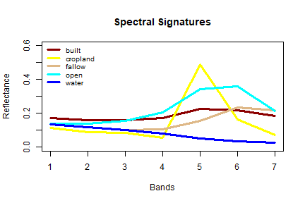
The spectral signatures (profile) shows (dis)similarity in the reflectance of different features on the earth’s surface (or above it). ‘Water’ shows relatively low reflection in all wavelengths, and ‘built’, ‘fallow’ and ‘open’ have relatively high reflectance in the longer wavelengts.