Tracks
Introduction
Points on great circles, etc.
Points on great circles
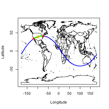
Points on a great circle are returned by the function ‘greatCircle’, using two points on the great circle to define it, and an additional argument to indicate how many points should be returned. You can also use greatCircleBearing, and provide starting points and bearing as arguments. gcIntermediate only returns points on the great circle that are on the track of shortest distance between the two points defining the great circle; and midPoint computes the point half-way between the two points. You can use onGreatCircle to test whether a point is on a great circle between two other points.
library(geosphere)
LA <- c(-118.40, 33.95)
NY <- c(-73.78,  40.63)
data(wrld)
plot(wrld, type='l')
gc <- greatCircle(LA, NY)
lines(gc, lwd=2, col='blue')
gci <- gcIntermediate(LA, NY)
lines(gci, lwd=4, col='green')
points(rbind(LA, NY), col='red', pch=20, cex=2)
mp <- midPoint(LA, NY)
onGreatCircle(LA,NY, rbind(mp,c(0,0)))
## [1] FALSE FALSE
points(mp, pch='*', cex=3, col='orange')
greatCircleBearing(LA, brng=270, n=10)
##        lon        lat
##  [1,] -144  31.210677
##  [2,] -108  33.532879
##  [3,]  -72  25.004950
##  [4,]  -36   5.254184
##  [5,]    0 -17.620746
##  [6,]   36 -31.210677
##  [7,]   72 -33.532879
##  [8,]  108 -25.004950
##  [9,]  144  -5.254184
## [10,]  180  17.620746
Maximum latitude on a great circle
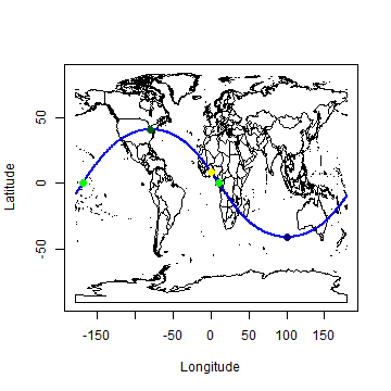
You can use the functions illustrated below to find out what the maximum latitude is that a great circle will reach; at what latitude it crosses a specified longitude; or at what longitude it crosses a specified latitude. From the map below it appears that Clairaut’s formula, used in gcMaxLat is not very accurate. Through optimization with function greatCircle, a more accurate value was found. The southern-most point is the antipode (a point at the opposite end of the world) of the northern-most point.
ml <- gcMaxLat(LA, NY)
lat0 <- gcLat(LA, NY, lon=0)
lon0 <- gcLon(LA, NY, lat=0)
plot(wrld, type='l')
lines(gc, lwd=2, col='blue')
points(ml, col='red', pch=20, cex=2)
points(cbind(0, lat0), pch=20, cex=2, col='yellow')
points(t(rbind(lon0, 0)), pch=20, cex=2, col='green' )
f <- function(lon){gcLat(LA, NY, lon)}
opt <- optimize(f, interval=c(-180, 180), maximum=TRUE)
points(opt$maximum, opt$objective, pch=20, cex=2, col='dark green' )
anti <- antipode(c(opt$maximum, opt$objective))
points(anti, pch=20, cex=2, col='dark blue' )
Great circle intersections
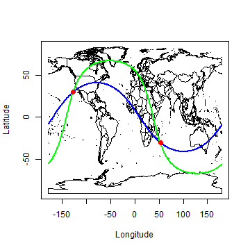
Points of intersection of two great circles can be computed in two ways. We use a second great circle that connects San Francisco with Amsterdam. We first compute where they cross by defining the great circles using two points on it (gcIntersect). After that, we compute the same points using a start point and initial bearing (gcIntersectBearing). The two points where the great circles cross are antipodes. Antipodes are connected with an infinite number of great circles.
SF <- c(-122.44, 37.74)
AM <- c(4.75, 52.31)
gc2 <- greatCircle(AM, SF)
plot(wrld, type='l')
lines(gc, lwd=2, col='blue')
lines(gc2, lwd=2, col='green')
int <- gcIntersect(LA, NY, SF, AM)
int
##          lon1      lat1      lon2     lat2
## [1,] 52.62562 -30.15099 -127.3744 30.15099
antipodal(int[,1:2], int[,3:4])
## [1] TRUE
points(rbind(int[,1:2], int[,3:4]), col='red', pch=20, cex=2)
bearing1 <- bearing(LA, NY)
bearing2 <- bearing(SF, AM)
bearing1
## [1] 65.93893
bearing2
## [1] 29.75753
gcIntersectBearing(LA, bearing1, SF, bearing2)
##           lon       lat       lon      lat
## [1,] 52.63076 -30.16041 -127.3692 30.16041