Direction
Introduction
Point at distance and bearing
Function destPoint returns the location of point given a point of origin, and a distance and bearing. Its perhaps obvious use in georeferencing locations of distant sitings. It can also be used to make circular polygons (with a fixed radius, but in longitude/latitude coordinates)
library(geosphere)
LA <- c(-118.40, 33.95)
NY <- c(-73.78, 40.63)
destPoint(LA, b=65, d=100000)
## lon lat
## [1,] -117.4152 34.32706
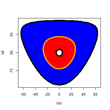
circle=destPoint(c(0,80), b=1:365, d=1000000)
circle2=destPoint(c(0,80), b=1:365, d=500000)
circle3=destPoint(c(0,80), b=1:365, d=100000)
plot(circle, type='l')
polygon(circle, col='blue', border='black', lwd=4)
polygon(circle2, col='red', lwd=4, border='orange')
polygon(circle3, col='white', lwd=4, border='black')
Triangulation
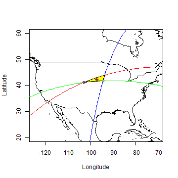
Below is triangulation example. We have three locations (NY, LA, MS) and three directions (281, 60, 195) towards a target. Because we are on a sphere, there are two (antipodal) results. We only show one here (by only using int[,1:2]). We compute the centroid from the polygon defined with the three points. To accurately draw a spherical polygon, we can use makePoly. This function inserts intermediate points along the paths between the vertices provided (default is one point every 10 km).
MS <- c(-93.26, 44.98)
gc1 <- greatCircleBearing(NY, 281)
gc2 <- greatCircleBearing(MS, 195)
gc3 <- greatCircleBearing(LA, 55)
data(wrld)
plot(wrld, type='l', xlim=c(-125, -70), ylim=c(20, 60))
lines(gc1, col='green')
lines(gc2, col='blue')
lines(gc3, col='red')
int <- gcIntersectBearing(rbind(NY, NY, MS),
            c(281, 281, 195), rbind(MS, LA, LA), c(195, 55, 55))
int
##             lon      lat      lon       lat
## [1,]  -94.40975 41.77229 85.59025 -41.77229
## [2,] -102.91692 41.15816 77.08308 -41.15816
## [3,]  -93.63298 43.97765 86.36702 -43.97765
distm(rbind(int[,1:2], int[,3:4]))
##            [,1]       [,2]       [,3]       [,4]       [,5]       [,6]
## [1,]        0.0   713665.0   253077.7 20003931.5 19308947.3 19751854.8
## [2,]   713665.0        0.0   823532.8 19308947.3 20003931.5 19195862.0
## [3,]   253077.7   823532.8        0.0 19751854.8 19195862.0 20003931.5
## [4,] 20003931.5 19308947.3 19751854.8        0.0   713665.0   253077.7
## [5,] 19308947.3 20003931.5 19195862.0   713665.0        0.0   823532.8
## [6,] 19751854.8 19195862.0 20003931.5   253077.7   823532.8        0.0
int <- int[,1:2]
points(int)
poly <- rbind(int, int[1,])
centr <- centroid(poly)
poly2 <- makePoly(int)
polygon(poly2, col='yellow')
points(centr, pch='*', col='dark red', cex=2)
Bearing
Below we first compute the distance and bearing from Los Angeles (LA) to New York (NY). These are then used to compute the point from LA at that distance in that (initial) bearing (direction). Bearing changes continuously when traveling along a Great Circle. The final bearing, when approaching NY, is also given.
d <- distCosine(LA, NY)
d
## [1] 3977614
b <- bearing(LA, NY)
b
## [1] 65.93893
destPoint(LA, b, d)
##            lon      lat
## [1,] -73.83063 40.63262
NY
## [1] -73.78  40.63
finalBearing(LA, NY)
## [1] 93.90995
Getting off-track
What if we went off-course and were flying over Minneapolis (MS)? The closest point on the planned route (p) can be computed with the alongTrackDistance and destPoint functions. The distance from ‘p’ to MS can be computed with the dist2gc (distance to great circle, or cross-track distance) function. The light green line represents the along-track distance, and the dark green line represents the cross-track distance.
atd <- alongTrackDistance(LA, NY, MS)
p <- destPoint(LA, b, atd)
plot(wrld, type='l', xlim=c(-130,-60), ylim=c(22,52))
gci <- gcIntermediate(LA, NY)
lines(gci, col='blue', lwd=2)
points(rbind(LA, NY), col='red', pch=20, cex=2)
points(MS[1], MS[2], pch=20, col='blue', cex=2)
lines(gcIntermediate(LA, p), col='green', lwd=3)
lines(gcIntermediate(MS, p), col='dark green', lwd=3)
points(p, pch=20, col='red', cex=2)
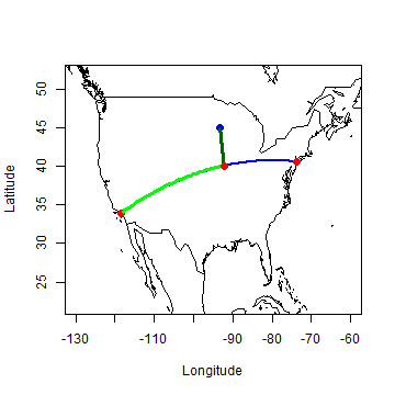
dist2gc(LA, NY, MS)
## [1] 549733.7
distCosine(p, MS)
## [1] 548738.9
Rhumb lines
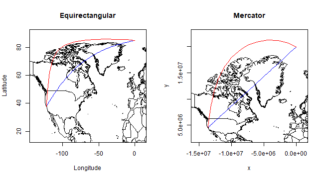
Rhumb (from the Spanish word for course, ‘rumbo’) lines are straight lines on a Mercator projection map (and at most latitudes pretty straight on an equirectangular projection (=unprojected lon/lat) map). They were used in navigation because it is easier to follow a constant compass bearing than to continually adjust direction as is needed to follow a great circle, even though rhumb lines are normally longer than great-circle (orthodrome) routes. Most rhumb lines will gradually spiral towards one of the poles.
NP <- c(0, 85)
SF <- c(-122.44, 37.74)
bearing(SF, NP)
## [1] 5.15824
b <- bearingRhumb(SF, NP)
b
## [1] 41.45714
dc <- distCosine(SF, NP)
dr <- distRhumb(SF, NP)
dc / dr
## [1] 0.8730767
pr <- destPointRhumb(SF, b, d=round(dr/100) * 1:100)
pc <- rbind(SF, gcIntermediate(SF, NP), NP)
par(mfrow=c(1,2))
plot(wrld, type='l', xlim=c(-140,10), ylim=c(15,90), main='Equirectangular')
lines(pr, col='blue')
lines(pc, col='red')
data(merc)
plot(merc, type='l', xlim=c(-15584729, 1113195),
                     ylim=c(2500000, 22500000), main='Mercator')
lines(mercator(pr), col='blue')
lines(mercator(pc), col='red')