Distance
Introduction
The geosphere package has six different functions to compute distance between two points with angular coordinates.
Three of these aproximate the earth as a sphere, these function
implement, in order of increasing complexity of the algorithm, the
‘Spherical law of cosines’, the ‘Haversine’ method (Sinnott, 1984) and
the ‘Vincenty Sphere’ method (Vincenty, 1975). The other three methods,
‘Vincenty Ellipsoid’ (Vincenty, 1975), Meeus, and Karney are based on an
ellipsoid (which is closer to the truth). For practical applications,
you should use the most precise method, to compute distances, which is
Karney’s method, as implemented in the distGeo function.
Spherical distance
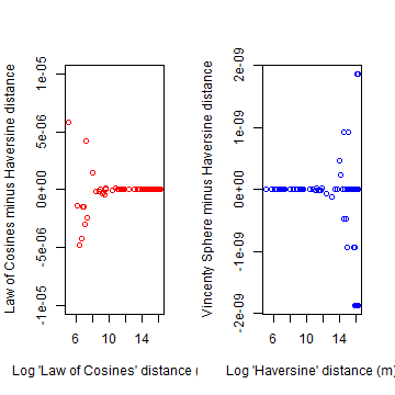
The results from the first three functions are identical for practical purposes. The Haversine (‘half-versed-sine’) formula was published by R.W. Sinnott in 1984, although it has been known for much longer. At that time computational precision was lower than today (15 digits precision). With current precision, the spherical law of cosines formula appears to give equally good results down to very small distances. If you want greater accuracy, you could use the distVincentyEllipsoid method.
Below the differences between the three spherical methods are illustrated. At very short distances, there are small differences between the ‘law of the Cosine’ and the other two methods. There are even smaller differences between the ‘Haversine’ and ‘Vincenty Sphere’ methods at larger distances.
library(geosphere)
##
## Attaching package: 'geosphere'
## The following object is masked from 'package:spatstat.geom':
##
##     perimeter
Lon = c(1:9/1000, 1:9/100, 1:9/10, 1:90*2)
Lat = c(1:9/1000, 1:9/100, 1:9/10, 1:90)
dcos = distCosine(c(0,0), cbind(Lon, Lat))
dhav = distHaversine(c(0,0), cbind(Lon, Lat))
dvsp = distVincentySphere(c(0,0), cbind(Lon, Lat))
par(mfrow=(c(1,2)))
plot(log(dcos), dcos-dhav, col='red', ylim=c(-1e-05, 1e-05),
            xlab="Log 'Law of Cosines' distance (m)",
            ylab="Law of Cosines minus Haversine distance")
plot(log(dhav), dhav-dvsp, col='blue',
            xlab="Log 'Haversine' distance (m)",
            ylab="Vincenty Sphere minus Haversine distance")
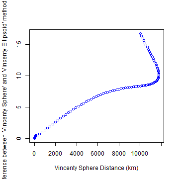
Geodetic distance
The difference with the ‘Vincenty Ellipsoid’ method is more pronounced. In the example below (using the default WGS83 ellipsoid), the difference is about 0.3% at very small distances, and 0.15% at larger distances.
dvse = distVincentyEllipsoid(c(0,0), cbind(Lon, Lat))
plot(dvsp/1000, (dvsp-dvse)/1000, col='blue', xlab='Vincenty Sphere Distance (km)',
        ylab="Difference between 'Vincenty Sphere' and 'Vincenty Ellipsoid' methods (km)")
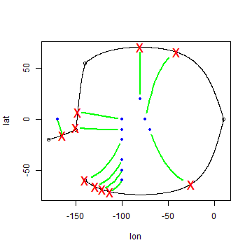
Distance to a polyline
The two function describe above are used in the dist2Line function that computes the shortest distance between a set of points and a set of spherical poly-lines (or polygons).
line <- rbind(c(-180,-20), c(-150,-10), c(-140,55), c(10, 0), c(-140,-60))
pnts <- rbind(c(-170,0), c(-75,0), c(-70,-10), c(-80,20), c(-100,-50),
           c(-100,-60), c(-100,-40), c(-100,-20), c(-100,-10), c(-100,0))
d = dist2Line(pnts, line)
plot( makeLine(line), type='l')
points(line)
points(pnts, col='blue', pch=20)
points(d[,2], d[,3], col='red', pch='x', cex=2)
for (i in 1:nrow(d)) lines(gcIntermediate(pnts[i,], d[i,2:3], 10), lwd=2, col='green')
References
Karney, C.F.F. GeographicLib.
Sinnott, R.W, 1984. Virtues of the Haversine. Sky and Telescope 68(2): 159
Vincenty, T. 1975. Direct and inverse solutions of geodesics on the ellipsoid with application of nested equations. Survey Review 23(176): 88-93. Available here.