Supervised Classification
Here we explore supervised classification. Various supervised classification algorithms exist, and the choice of algorithm can affect the results. Here we explore two related algorithms (CART and RandomForest).
In supervised classification, we have prior knowledge about some of the land-cover types through, for example, fieldwork, reference spatial data or interpretation of high resolution imagery (such as available on Google maps). Specific sites in the study area that represent homogeneous examples of these known land-cover types are identified. These areas are commonly referred to as training sites because the spectral properties of these sites are used to train the classification algorithm.
The following examples uses a Classification and Regression Trees (CART) classifier (Breiman et al. 1984) (further reading to predict land use land cover classes in the study area.
We will perform the following steps:
Generate sample sites based on a reference raster
Extract cell values from Landsat data for the sample sites
Train the classifier using training samples
Classify the Landsat data using the trained model
Evaluate the accuracy of the model
Reference data
The National Land Cover Database 2011 (NLCD 2011) is a land cover product for the USA. NLCD is a 30-m Landsat-based land cover database spanning 4 epochs (1992, 2001, 2006 and 2011). NLCD 2011 is based primarily on a decision-tree classification of circa 2011 Landsat data.
You can find the class names in NCLD 2011 (here)[https://www.mrlc.gov/nlcd11_leg.php]. It has two pairs of class values and names that correspond to the levels of land use and land cover classification system. These levels usually represent the level of complexity, level I being the simplest with broad land use land cover categories. Read this report by Anderson et al to learn more about this land use and land cover classification system.
library(raster)
nlcd <- brick('data/rs/nlcd-L1.tif')
names(nlcd) <- c("nlcd2001", "nlcd2011")
# The class names and colors for plotting
nlcdclass <- c("Water", "Developed", "Barren", "Forest", "Shrubland", "Herbaceous", "Planted/Cultivated", "Wetlands")
classdf <- data.frame(classvalue1 = c(1,2,3,4,5,7,8,9), classnames1 = nlcdclass)
# Hex codes of colors
classcolor <- c("#5475A8", "#B50000", "#D2CDC0", "#38814E", "#AF963C", "#D1D182", "#FBF65D", "#C8E6F8")
# Now we ratify (RAT = "Raster Attribute Table") the ncld2011 (define RasterLayer as a categorical variable). This is helpful for plotting.
nlcd2011 <- nlcd[[2]]
nlcd2011 <- ratify(nlcd2011)
rat <- levels(nlcd2011)[[1]]
#
rat$landcover <- nlcdclass
levels(nlcd2011) <- rat
We did a lot of things here. Take a step back and read more about
ratify.
Note There is no class with value 6.
Generate sample sites
As we discussed in the class, training and/or validation data can come from a variety of sources. In this example we will generate the training and validation sample sites using the NLCD reference RasterLayer. Alternatively, you can use predefined sites that you may have collected from other sources. We will generate the sample sites following a stratified random sampling to ensure samples from each LULC class.
# Load the training sites locations
# Set the random number generator to reproduce the results
set.seed(99)
# Sampling
samp2011 <- sampleStratified(nlcd2011, size = 200, na.rm = TRUE, sp = TRUE)
samp2011
## class       : SpatialPointsDataFrame
## features    : 1600
## extent      : -121.9257, -121.4225, 37.85415, 38.18536  (xmin, xmax, ymin, ymax)
## crs         : +proj=longlat +datum=WGS84 +no_defs
## variables   : 2
## names       :    cell, nlcd2011
## min values  :     413,        1
## max values  : 2307837,        9
# Number of samples in each class
table(samp2011$nlcd2011)
##
##   1   2   3   4   5   7   8   9
## 200 200 200 200 200 200 200 200
You can see there are two variables in samp2011. The cell column
contains cell numbers of nlcd2011 sampled. nlcd2011 column
contains the class values (1-9). We will drop the cell column later.
Here nlcd has integer values between 1-9. You will often find
classnames are provided as string labels (e.g. water, crop, vegetation).
You will need to ‘relabel’ class names to integer or factors if only
string labels are supplied before using them as response variable in the
classification. There are several approaches that could be used to
convert these classes to integer codes. We can make a function that will
reclassify the character strings representing land cover classes into
integers based on the existing factor levels.
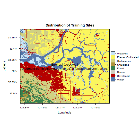
Let’s plot the training sites over the nlcd2011 RasterLayer to
visualize the distribution of sampling locations.
library(rasterVis)
plt <- levelplot(nlcd2011, col.regions = classcolor, main = 'Distribution of Training Sites')
print(plt + layer(sp.points(samp2011, pch = 3, cex = 0.5, col = 1)))
rasterVis offers more advanced (trellis/lattice) plotting of
Raster* objects. Please install the package if it is not available for
your machine.
Extract values for sites
Here is our Landsat data.
landsat5 <- stack('data/rs/centralvalley-2011LT5.tif')
names(landsat5) <- c('blue', 'green', 'red', 'NIR', 'SWIR1', 'SWIR2')
Once we have the sites, we can extract the cell values from landsat5
RasterStack. These band values will be the predictor variables and
“classvalues” from nlcd2011 will be the response variable.
# Extract the layer values for the locations
sampvals <- extract(landsat5, samp2011, df = TRUE)
# sampvals no longer has the spatial information. To keep the spatial information you use `sp=TRUE` argument in the `extract` function.
# drop the ID column
sampvals <- sampvals[, -1]
# combine the class information with extracted values
sampdata <- data.frame(classvalue = samp2011@data$nlcd2011, sampvals)
Train the classifier
Now we will train the classification algorithm using training2011
dataset.
library(rpart)
# Train the model
cart <- rpart(as.factor(classvalue)~., data=sampdata, method = 'class', minsplit = 5)
# print(model.class)
# Plot the trained classification tree
plot(cart, uniform=TRUE, main="Classification Tree")
text(cart, cex = 0.8)
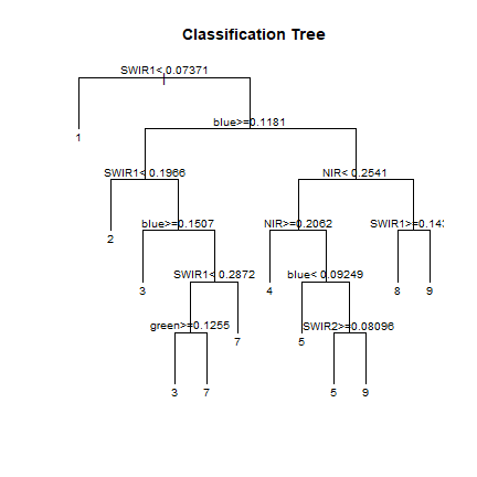
In the classification tree plot classvalues are printed at the leaf
nodes. You can find the corresponding land use land cover names from the
classdf data.frame.
See ?rpart.control to set different parameters for building the
model.
You can print/plot more about the cart model created in the previous
example. E.g. you can use plotcp(cart) to learn about the
cost-complexity (cp argument in rpart).
Classify
Now we have our trained classification model (cart), we can use it
to make predictions, that is, to classify all cells in the landsat5
RasterStack.
Important The names in the Raster object to be classified should exactly match those expected by the model. This will be the case if the same Raster object was used (via extract) to obtain the values to fit the model.
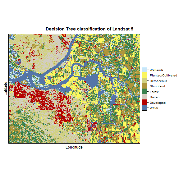
# Now predict the subset data based on the model; prediction for entire area takes longer time
pr2011 <- predict(landsat5, cart, type='class')
pr2011
## class      : RasterLayer
## dimensions : 1230, 1877, 2308710  (nrow, ncol, ncell)
## resolution : 0.0002694946, 0.0002694946  (x, y)
## extent     : -121.9258, -121.42, 37.85402, 38.1855  (xmin, xmax, ymin, ymax)
## crs        : +proj=longlat +datum=WGS84 +no_defs
## source     : memory
## names      : layer
## values     : 1, 9  (min, max)
## attributes :
##        ID value
##  from:  1     1
##   to :  8     9
Now plot the classification result using rasterVis. See will set the
classnames for the classvalues.
pr2011 <- ratify(pr2011)
rat <- levels(pr2011)[[1]]
rat$legend <- classdf$classnames
levels(pr2011) <- rat
levelplot(pr2011, maxpixels = 1e6,
          col.regions = classcolor,
          scales=list(draw=FALSE),
          main = "Decision Tree classification of Landsat 5")
Question 1:Plot ``nlcd2011`` and ``pr2011`` side-by-side and comment about the accuracy of the prediction (e.g. mixing between cultivated crops, pasture, grassland and shrubs).
You may need to select more samples and use additional predictor variables. The choice of classifier also plays an important role.
Model evaluation
Now let’s assess the accuracy of the model to get an idea of how
accurate the classified map might be. Two widely used measures in remote
sensing are “overall accuracy” and “kappa”. You can perform the accuracy
assessment using the independent samples (validation2011).
To evaluate any model, you can use k-fold cross-validation. In this
technique the data used to fit the model is split into k groups
(typically 5 groups). In turn, one of the groups will be used for model
testing, while the rest of the data is used for model training
(fitting).
library(dismo)
set.seed(99)
j <- kfold(sampdata, k = 5, by=sampdata$classvalue)
table(j)
## j
##   1   2   3   4   5
## 320 320 320 320 320
Now we train and test the model five times, each time computing a confusion matrix that we store in a list.
x <- list()
for (k in 1:5) {
    train <- sampdata[j!= k, ]
    test <- sampdata[j == k, ]
    cart <- rpart(as.factor(classvalue)~., data=train, method = 'class', minsplit = 5)
    pclass <- predict(cart, test, type='class')
    # create a data.frame using the reference and prediction
    x[[k]] <- cbind(test$classvalue, as.integer(pclass))
}
Now combine the five list elements into a single data.frame, using
do.call and compute a confusion matrix.
y <- do.call(rbind, x)
y <- data.frame(y)
colnames(y) <- c('observed', 'predicted')
conmat <- table(y)
# change the name of the classes
colnames(conmat) <- classdf$classnames
rownames(conmat) <- classdf$classnames
conmat
##                     predicted
## observed             Water Developed Barren Forest Shrubland Herbaceous
##   Water                175         6      0      3         0          0
##   Developed              2        90     51      8        10         22
##   Barren                 7        39     82      4        19         38
##   Forest                 0         2      1    106        57          1
##   Shrubland              0         3      5     59       102         12
##   Herbaceous             0         9     36     10        27        109
##   Planted/Cultivated     0         7     11     34        42         19
##   Wetlands              18        10      6     36        29          5
##                     predicted
## observed             Planted/Cultivated Wetlands
##   Water                               7        9
##   Developed                          11        6
##   Barren                              5        6
##   Forest                              6       27
##   Shrubland                          12        7
##   Herbaceous                          8        1
##   Planted/Cultivated                 69       18
##   Wetlands                           33       63
Question 2:Comment on the miss-classification between different classes.
Question 3:Can you think of ways to to improve the accuracy.
Compute the overall accuracy and the “Kappa” statistic.
Overall accuracy:
# number of cases
n <- sum(conmat)
n
## [1] 1600
# number of correctly classified cases per class
diag <- diag(conmat)
# Overall Accuracy
OA <- sum(diag) / n
OA
## [1] 0.4975
Kappa:
# observed (true) cases per class
rowsums <- apply(conmat, 1, sum)
p <- rowsums / n
# predicted cases per class
colsums <- apply(conmat, 2, sum)
q <- colsums / n
expAccuracy <- sum(p*q)
kappa <- (OA - expAccuracy) / (1 - expAccuracy)
kappa
## [1] 0.4257143
Producer and user accuracy
# Producer accuracy
PA <- diag / colsums
# User accuracy
UA <- diag / rowsums
outAcc <- data.frame(producerAccuracy = PA, userAccuracy = UA)
outAcc
##                    producerAccuracy userAccuracy
## Water                     0.8663366        0.875
## Developed                 0.5421687        0.450
## Barren                    0.4270833        0.410
## Forest                    0.4076923        0.530
## Shrubland                 0.3566434        0.510
## Herbaceous                0.5291262        0.545
## Planted/Cultivated        0.4569536        0.345
## Wetlands                  0.4598540        0.315
Question 4:Perform the classification using Random Forest classifiers from the ``randomForest`` package
Question 5:Plot the results of rpart and Random Forest classifier side-by-side.
Question 6 (optional):Repeat the steps for the year 2001 using
Random Forest. Use the cloud-free composite image
data/centralvalley-2001LE7.tif. This is Landsat
7 data . Use as reference
data the National Land Cover Database 2001 (NLCD
2001) for the subset of the
California Central Valley.*
Question 7 (optional):We have trained the classifiers using 200 samples for each class. Investigate the effect of sample size on classification. Repeat the steps with different subsets, e.g. a sample size of 150, 100, 50 per class, and compare the results. Use the same holdout samples for model evaluation.