Unsupervised Classification
In this chapter we explore unsupervised classification. Various unsupervised classification algorithms exist, and the choice of algorithm can affect the results. We will explore only one algorithm (k-means) to illustrate the general principle.
For this example, we will follow the National Land Cover Database 2011 (NLCD 2011) classification scheme for a subset of the Central Valley regions. We use cloud-free composite image from Landsat 5 with 6 bands.
library(raster)
landsat5 <- stack('data/rs/centralvalley-2011LT5.tif')
names(landsat5) <- c('blue', 'green', 'red', 'NIR', 'SWIR1', 'SWIR2')
Question 1: Make a 3-band False Color Composite plot of ``landsat5``.
In unsupervised classification, we use the reflectance data, but we don’t supply any response data (that is, we do not identify any pixel as belonging to a particular class). This may seem odd, but it can be useful when we don’t have much prior knowledge of a study area. Or if you have broad knowledge of the distribution of land cover classes of interest, but no specific ground data.
The algorithm groups pixels with similar spectral characteristics into groups.
Learn more about K-means and other unsupervised-supervised algorithms here.
We will perform unsupervised classification on a spatial subset of the
ndvi layer. Here is yet another way to compute ndvi. In this case we
do not use a separate function, but we use a direct algebraic notation.
ndvi <- (landsat5[['NIR']] - landsat5[['red']]) / (landsat5[['NIR']] + landsat5[['red']])
We will do kmeans clustering of the ndvi data. First we use
crop to make a spatial subset of the ndvi, to allow for faster
processing (you can select any extent using the drawExtent()
function).
kmeans classification
# Extent to crop ndvi layer
e <- extent(-121.807, -121.725, 38.004, 38.072)
# crop landsat by the extent
ndvi <- crop(ndvi, e)
ndvi
## class      : RasterLayer
## dimensions : 252, 304, 76608  (nrow, ncol, ncell)
## resolution : 0.0002694946, 0.0002694946  (x, y)
## extent     : -121.807, -121.725, 38.00413, 38.07204  (xmin, xmax, ymin, ymax)
## crs        : +proj=longlat +datum=WGS84 +no_defs
## source     : memory
## names      : layer
## values     : -0.3360085, 0.7756007  (min, max)
# convert the raster to vecor/matrix
nr <- getValues(ndvi)
str(nr)
##  num [1:76608] 0.245 0.236 0.272 0.277 0.277 ...
Please note that getValues converted the ndvi RasterLayer to an
array (matrix). Now we will perform the kmeans clustering on the
matrix and inspect the output.
# It is important to set the seed generator because `kmeans` initiates the centers in random locations
set.seed(99)
# We want to create 10 clusters, allow 500 iterations, start with 5 random sets using "Lloyd" method
kmncluster <- kmeans(na.omit(nr), centers = 10, iter.max = 500, nstart = 5, algorithm="Lloyd")
# kmeans returns an object of class "kmeans"
str(kmncluster)
## List of 9
##  $ cluster     : int [1:76608] 4 4 3 3 3 3 3 4 4 4 ...
##  $ centers     : num [1:10, 1] 0.55425 0.00498 0.29997 0.20892 -0.20902 ...
##   ..- attr(*, "dimnames")=List of 2
##   .. ..$ : chr [1:10] "1" "2" "3" "4" ...
##   .. ..$ : NULL
##  $ totss       : num 6459
##  $ withinss    : num [1:10] 5.69 6.13 4.91 4.9 5.75 ...
##  $ tot.withinss: num 55.8
##  $ betweenss   : num 6403
##  $ size        : int [1:10] 8932 4550 7156 6807 11672 8624 8736 5040 9893 5198
##  $ iter        : int 108
##  $ ifault      : NULL
##  - attr(*, "class")= chr "kmeans"
kmeans returns an object with 9 elements. The length of the
cluster element within kmncluster is 76608 which same as length
of nr created from the ndvi. The cell values of
kmncluster$cluster range between 1 to 10 corresponding to the input
number of cluster we provided in the kmeans function.
kmncluster$cluster indicates the cluster label for corresponding
pixel. We need to convert the kmncluster$cluster values back to
RasterLayer of the same dimension as the ndvi.
# Use the ndvi object to set the cluster values to a new raster
knr <- setValues(ndvi, kmncluster$cluster)
# You can also do it like this
knr <- raster(ndvi)
values(knr) <- kmncluster$cluster
knr
## class      : RasterLayer
## dimensions : 252, 304, 76608  (nrow, ncol, ncell)
## resolution : 0.0002694946, 0.0002694946  (x, y)
## extent     : -121.807, -121.725, 38.00413, 38.07204  (xmin, xmax, ymin, ymax)
## crs        : +proj=longlat +datum=WGS84 +no_defs
## source     : memory
## names      : layer
## values     : 1, 10  (min, max)
We can see that knr is a RasterLayer but we do not know which
cluster (1-10) belongs to what land cover class (and if it does belong
to a class that we would recognize). You can find that out by plotting
them side-by-side with a reference layers and using unique color for
each cluster.
# Define a color vector for 10 clusters (learn more about setting the color later)
mycolor <- c("#fef65b","#ff0000", "#daa520","#0000ff","#0000ff","#00ff00","#cbbeb5",
             "#c3ff5b", "#ff7373", "#00ff00", "#808080")
par(mfrow = c(1,2))
plot(ndvi, col = rev(terrain.colors(10)), main = 'Landsat-NDVI')
plot(knr, main = 'Unsupervised classification', col = mycolor )
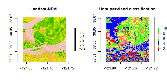
While for other purposes it is usually better to define more classes (and possibly merge classes later), a simple classification like this one could be useful, e.g., merge cluster 4 and 5 to construct a water mask for the year 2011.
You can change the colors in my mycolor. Learn more about selecting
colors in R
here
and
here.
Question 2:Plot 3-band RGB of ``landsat5`` for the subset (extent ``e``) and result of ``kmeans`` clustering side-by-side and make a table of land-use land-cover labels for the clusters. E.g. cluster 4 and 5 are water.