2. The length of a coastline¶

How Long Is the Coast of Britain? Statistical Self-Similarity and Fractional Dimension is the title of a famous paper by Benoît Mandelbrot. Mandelbrot uses data from a paper by Lewis Fry Richardson who showed that the length of a coastline changes with scale, or, more precisely, with the length (resolution) of the measuring stick (ruler) used. Mandelbrot discusses the fractal dimension D of such lines. D is 1 for a straight line, and higher for more wrinkled shapes. For the west coast of Britain, Mandelbrot reports that D=1.25. Here I show how to measure the length of a coast line with rulers of different length and how to compute a fractal dimension.

First we get a high spatial resolution (30 m) coastline for the United Kingdom from the GADM database.

library(raster)
uk <- raster::getData('GADM', country='GBR', level=0)
par(mai=c(0,0,0,0))
plot(uk)

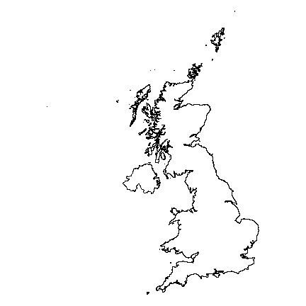
This is a single ‘multi-polygon’ (it has a single feature) and a longitude/latitude coordinate reference system.

data.frame(uk)
##   GID_0         NAME_0
## 1   GBR United Kingdom

Let’s transform this to a planar coordinate system. That is not required, but it will speed up computations. We used a the Transverse Mercator (tmerc) projection similar to the “British National Grid”.

prj <- "+proj=tmerc +lat_0=49 +lon_0=-2 +k=0.9996012717 +x_0=400000 +y_0=-100000 +datum=WGS84 +units=m"

Note that the units are meters.

With that we can transform the coordinates of uk from longitude latitude to the British National Grid.

library(rgdal)
guk <- spTransform(uk, CRS(prj))

We only want the main island, so want need to separate (disaggregate) the different polygons.

duk <- disaggregate(guk)
head(duk)
##   GID_0         NAME_0
## 1   GBR United Kingdom
## 2   GBR United Kingdom
## 3   GBR United Kingdom
## 4   GBR United Kingdom
## 5   GBR United Kingdom
## 6   GBR United Kingdom

Now we have 920 features. We want the largest one.

a <- area(duk)
i <- which.max(a)
a[i] / 1000000
## [1] 219143.4
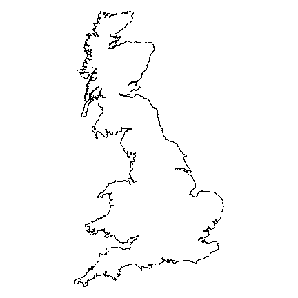
b <- duk[i,]

Britain has an area of about 220,000 km².

par(mai=rep(0,4))
plot(b)

On to the tricky part. The function to go around the coast with a ruler (yardstick) of a certain length.

measure_with_ruler <- function(pols, length, lonlat=FALSE) {
    # some sanity checking
    stopifnot(inherits(pols, 'SpatialPolygons'))
    stopifnot(length(pols) == 1)
    # get the coordinates of the polygon
    g <- geom(pols)[, c('x', 'y')]
    nr <- nrow(g)
    # we start at the first point
    pts <- 1
    newpt <- 1
    while(TRUE) {
        # start here
        p <- newpt
        # order the points
        j <- p:(p+nr-1)
        j[j > nr] <- j[j > nr] - nr
        gg <- g[j,]
        # compute distances
        pd <- pointDistance(gg[1,], gg, lonlat)
        # get the first point that is past the end of the ruler
        # this is precise enough for our high resolution coastline
        i <- which(pd > length)[1]
        if (is.na(i)) {
            stop('Ruler is longer than the maximum distance found')
        }
        # get the record number for new point in the original order
        newpt <- i + p
        # stop if past the last point
        if (newpt >= nr) break
        pts <- c(pts, newpt)
    }
    # add the last (incomplete) stick.
    pts <- c(pts, 1)
    # return the locations
    g[pts, ]
}

Now we have the function, life is easy, we just call it a couple of times, using rulers of different lengths.

y <- list()
rulers <- c(25,50,100,150,200,250) # km
for (i in 1:length(rulers)) {
    y[[i]] <- measure_with_ruler(b, rulers[i]*1000)
}

Object y is a list of matrices containing the locations where the ruler touched the coast. We can plot these on top of a map of Britain.

par(mfrow=c(2,3), mai=rep(0,4))
for (i in 1:length(y)) {
    plot(b, col='lightgray', lwd=2)
    p <- y[[i]]
    lines(p, col='red', lwd=3)
    points(p, pch=20, col='blue', cex=2)
    bar <- rbind(cbind(525000, 900000), cbind(525000, 900000-rulers[i]*1000))
    lines(bar, lwd=2)
    points(bar, pch=20, cex=1.5)
    text(525000, mean(bar[,2]), paste(rulers[i], '  km'), cex=1.5)
    text(525000, bar[2,2]-50000, paste0('(', nrow(p), ')'), cex=1.25)
}

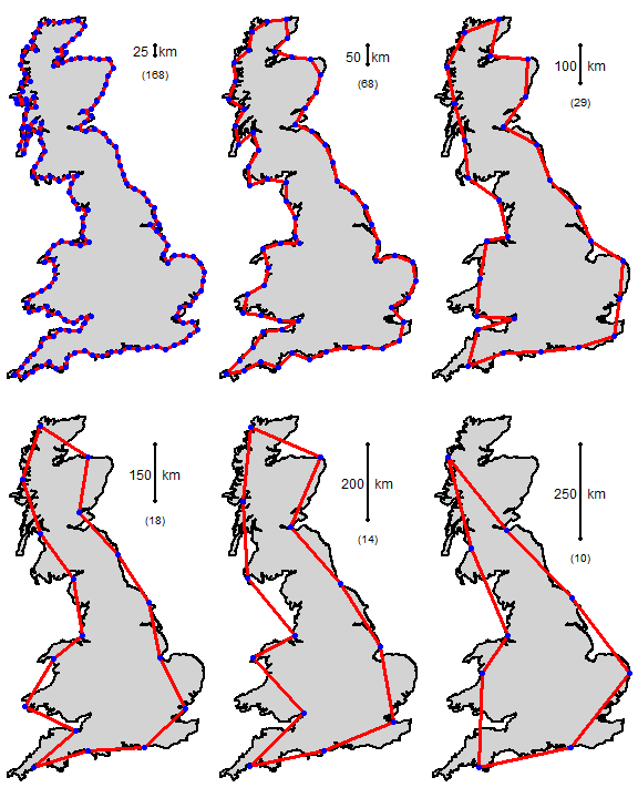
The coastline of Britain, measured with rulers of different lengths. The number of segments is in parenthesis. f

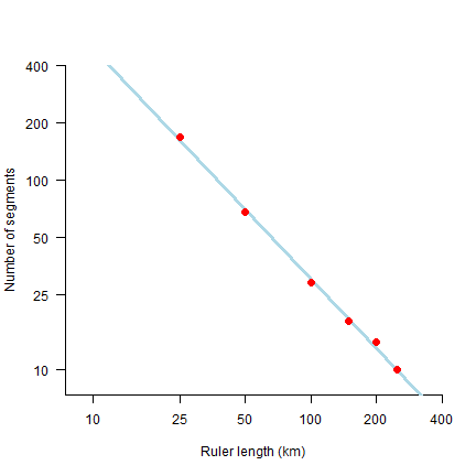
Here is the fractal (log-log) plot. Note how the axes are on the log scale, but that I used the non-transformed values for the labels.

# number of times a ruler was used
n <- sapply(y, nrow)
# set up empty plot
plot(log(rulers), log(n), type='n', xlim=c(2,6), ylim=c(2,6), axes=FALSE,
       xaxs="i",yaxs="i", xlab='Ruler length (km)', ylab='Number of segments')
# axes
tics <- c(1,10,25,50,100,200,400)
axis(1, at=log(tics), labels=tics)
axis(2, at=log(tics), labels=tics, las=2)
# linear regression line
m <- lm(log(n)~log(rulers))
abline(m, lwd=3, col='lightblue')
# add observations
points(log(rulers), log(n), pch=20, cex=2, col='red')

What does this mean? Let’s try some very small rulers, from 1 mm to 10 m.

small_rulers <- c(0.000001, 0.00001, 0.0001, 0.001, 0.01)  # km
nprd <- exp(predict(m, data.frame(rulers=small_rulers)))
coast <- nprd * small_rulers
plot(small_rulers, coast, xlab='Length of ruler', ylab='Length of coast', pch=20, cex=2, col='red')

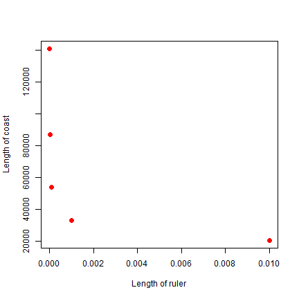
So as the ruler get smaller, the coastline gets exponentially longer. As the ruler approaches zero, the length of the coastline approaches infinity.

The fractal dimension D of the coast of Britain is the (absolute value of the) slope of the regression line.

m
##
## Call:
## lm(formula = log(n) ~ log(rulers))
##
## Coefficients:
## (Intercept)  log(rulers)
##       8.976       -1.208

Get the slope

-1 * m$coefficients[2]
## log(rulers)
##    1.208451

Very close to Mandelbrot’s D = 1.25 for the west coast of Britain.