Vector data
Introduction
Package sp is the central package supporting spatial data analysis
in R. sp defines a set of classes to represent spatial data. A
class defines a particular data type. The data.frame is an example
of a class. Any particular data.frame you create is an object
(instantiation) of that class.
The main reason for defining classes is to create a standard
representation of a particular data type to make it easier to write
functions (also known as ‘methods’) for them. In fact, the sp
package does not provide many functions to modify or analyze spatial
data; but the classes it defines are used in more than 100 other R
packages that provide specific functionality. See Hadley Wickham’s
Advanced R or John Chambers’ Software for
data analysis for a
detailed discussion of the use of classes in R).
We will be using the sp package here. Note that this package will
eventually be replaced by the newer sf package — but sp is still
more commonly used.
Package sp introduces a number of classes with names that start with
Spatial. For vector data, the basic types are the SpatialPoints,
SpatialLines, and SpatialPolygons. These classes only represent
geometries. To also store attributes, classes are available with these
names plus DataFrame, for example, SpatialPolygonsDataFrame and
SpatialPointsDataFrame. When referring to any object with a name
that starts with Spatial, it is common to write Spatial*. When
referring to a SpatialPolygons or SpatialPolygonsDataFrame
object it is common to write SpatialPolygons*. The Spatial
classes (and their use) are described in detail by Bivand, Pebesma and
Gómez-Rubio.
It is possible to create Spatial* objects from scratch with R
code. It can be very useful to create small self contained example to
illustrate something, for example to ask a question about how to do a
particular operation without needing to give access to the real data you
are using (which is always cumbersome). But in real life you will read
these from a file or database, for example from a “shapefile” see
Chapter 5.
To get started, let’s make some Spatial objects from scratch anyway, using the same data as were used in the previous chapter.
SpatialPoints
longitude <- c(-116.7, -120.4, -116.7, -113.5, -115.5, -120.8, -119.5, -113.7, -113.7, -110.7)
latitude <- c(45.3, 42.6, 38.9, 42.1, 35.7, 38.9, 36.2, 39, 41.6, 36.9)
lonlat <- cbind(longitude, latitude)
Now create a SpatialPoints object. First load the sp package
from the library. If this command fails with
Error in library(sp) : there is no package called ‘sp’, then you
need to install the package first, with install.packages("sp")
library(sp)
pts <- SpatialPoints(lonlat)
Let’s check what kind of object pts is.
class (pts)
## [1] "SpatialPoints"
## attr(,"package")
## [1] "sp"
And what is inside of it
showDefault(pts)
## An object of class "SpatialPoints"
## Slot "coords":
##       longitude latitude
##  [1,]    -116.7     45.3
##  [2,]    -120.4     42.6
##  [3,]    -116.7     38.9
##  [4,]    -113.5     42.1
##  [5,]    -115.5     35.7
##  [6,]    -120.8     38.9
##  [7,]    -119.5     36.2
##  [8,]    -113.7     39.0
##  [9,]    -113.7     41.6
## [10,]    -110.7     36.9
##
## Slot "bbox":
##              min    max
## longitude -120.8 -110.7
## latitude    35.7   45.3
##
## Slot "proj4string":
## Coordinate Reference System:
## Deprecated Proj.4 representation: NA
So we see that the object has the coordinates we supplied, but also a
bbox. This is a ‘bounding box’, or the ‘spatial extent’ that was
computed from the coordinates. There is also a “proj4string”. This
stores the coordinate reference system (“crs”, discussed in more detail
later). We did not provide the crs so it is unknown (NA). That is
not good, so let’s recreate the object, and now provide a crs.
crdref <- CRS('+proj=longlat +datum=WGS84')
pts <- SpatialPoints(lonlat, proj4string=crdref)
I load to raster package to improve how Spatial objects are printed.
library(raster)
pts
## class       : SpatialPoints
## features    : 10
## extent      : -120.8, -110.7, 35.7, 45.3  (xmin, xmax, ymin, ymax)
## crs         : +proj=longlat +datum=WGS84 +no_defs
We can use the SpatialPoints object to create a
SpatialPointsDataFrame object. First we need a data.frame with
the same number of rows as there are geometries.
# Generate random precipitation values, same quantity as points
precipvalue <- runif(nrow(lonlat), min=0, max=100)
df <- data.frame(ID=1:nrow(lonlat), precip=precipvalue)
Combine the SpatialPoints with the data.frame.
ptsdf <- SpatialPointsDataFrame(pts, data=df)
ptsdf
## class       : SpatialPointsDataFrame
## features    : 10
## extent      : -120.8, -110.7, 35.7, 45.3  (xmin, xmax, ymin, ymax)
## crs         : +proj=longlat +datum=WGS84 +no_defs
## variables   : 2
## names       : ID,           precip
## min values  :  1, 6.17862704675645
## max values  : 10, 99.1906094830483
To see what is inside:
str(ptsdf)
## Formal class 'SpatialPointsDataFrame' [package "sp"] with 5 slots
##   ..@ data       :'data.frame':  10 obs. of  2 variables:
##   .. ..$ ID    : int [1:10] 1 2 3 4 5 6 7 8 9 10
##   .. ..$ precip: num [1:10] 6.18 20.6 17.66 68.7 38.41 ...
##   ..@ coords.nrs : num(0)
##   ..@ coords     : num [1:10, 1:2] -117 -120 -117 -114 -116 ...
##   .. ..- attr(*, "dimnames")=List of 2
##   .. .. ..$ : NULL
##   .. .. ..$ : chr [1:2] "longitude" "latitude"
##   ..@ bbox       : num [1:2, 1:2] -120.8 35.7 -110.7 45.3
##   .. ..- attr(*, "dimnames")=List of 2
##   .. .. ..$ : chr [1:2] "longitude" "latitude"
##   .. .. ..$ : chr [1:2] "min" "max"
##   ..@ proj4string:Formal class 'CRS' [package "sp"] with 1 slot
##   .. .. ..@ projargs: chr "+proj=longlat +datum=WGS84 +no_defs"
##   .. .. ..$ comment: chr "GEOGCRS[\"unknown\",\n    DATUM[\"World Geodetic System 1984\",\n        ELLIPSOID[\"WGS 84\",6378137,298.25722"| __truncated__
Or
showDefault(ptsdf)
## An object of class "SpatialPointsDataFrame"
## Slot "data":
##    ID    precip
## 1   1  6.178627
## 2   2 20.597457
## 3   3 17.655675
## 4   4 68.702285
## 5   5 38.410372
## 6   6 76.984142
## 7   7 49.769924
## 8   8 71.761851
## 9   9 99.190609
## 10 10 38.003518
##
## Slot "coords.nrs":
## numeric(0)
##
## Slot "coords":
##       longitude latitude
##  [1,]    -116.7     45.3
##  [2,]    -120.4     42.6
##  [3,]    -116.7     38.9
##  [4,]    -113.5     42.1
##  [5,]    -115.5     35.7
##  [6,]    -120.8     38.9
##  [7,]    -119.5     36.2
##  [8,]    -113.7     39.0
##  [9,]    -113.7     41.6
## [10,]    -110.7     36.9
##
## Slot "bbox":
##              min    max
## longitude -120.8 -110.7
## latitude    35.7   45.3
##
## Slot "proj4string":
## Coordinate Reference System:
## Deprecated Proj.4 representation: +proj=longlat +datum=WGS84 +no_defs
## WKT2 2019 representation:
## GEOGCRS["unknown",
##     DATUM["World Geodetic System 1984",
##         ELLIPSOID["WGS 84",6378137,298.257223563,
##             LENGTHUNIT["metre",1]],
##         ID["EPSG",6326]],
##     PRIMEM["Greenwich",0,
##         ANGLEUNIT["degree",0.0174532925199433],
##         ID["EPSG",8901]],
##     CS[ellipsoidal,2],
##         AXIS["longitude",east,
##             ORDER[1],
##             ANGLEUNIT["degree",0.0174532925199433,
##                 ID["EPSG",9122]]],
##         AXIS["latitude",north,
##             ORDER[2],
##             ANGLEUNIT["degree",0.0174532925199433,
##                 ID["EPSG",9122]]]]
SpatialLines and SpatialPolygons
Making a SpatialPoints object was easy. Making a SpatialLines
and SpatialPolygons object is a bit harder, but stil relatively
straightforward with the spLines and spPolygons functions (from
the raster package).
lon <- c(-116.8, -114.2, -112.9, -111.9, -114.2, -115.4, -117.7)
lat <- c(41.3, 42.9, 42.4, 39.8, 37.6, 38.3, 37.6)
lonlat <- cbind(lon, lat)
lns <- spLines(lonlat, crs=crdref)
lns
## class       : SpatialLines
## features    : 1
## extent      : -117.7, -111.9, 37.6, 42.9  (xmin, xmax, ymin, ymax)
## crs         : +proj=longlat +datum=WGS84 +no_defs
pols <- spPolygons(lonlat, crs=crdref)
pols
## class       : SpatialPolygons
## features    : 1
## extent      : -117.7, -111.9, 37.6, 42.9  (xmin, xmax, ymin, ymax)
## crs         : +proj=longlat +datum=WGS84 +no_defs
The structure of the SpatialPolygons class is somewhat complex as it needs to accommodate the possibility of multiple polygons, each consisting of multiple sub-polygons, some of which may be “holes”.
str(pols)
## Formal class 'SpatialPolygons' [package "sp"] with 4 slots
##   ..@ polygons   :List of 1
##   .. ..$ :Formal class 'Polygons' [package "sp"] with 5 slots
##   .. .. .. ..@ Polygons :List of 1
##   .. .. .. .. ..$ :Formal class 'Polygon' [package "sp"] with 5 slots
##   .. .. .. .. .. .. ..@ labpt  : num [1:2] -114.7 40.1
##   .. .. .. .. .. .. ..@ area   : num 19.7
##   .. .. .. .. .. .. ..@ hole   : logi FALSE
##   .. .. .. .. .. .. ..@ ringDir: int 1
##   .. .. .. .. .. .. ..@ coords : num [1:8, 1:2] -117 -114 -113 -112 -114 ...
##   .. .. .. ..@ plotOrder: int 1
##   .. .. .. ..@ labpt    : num [1:2] -114.7 40.1
##   .. .. .. ..@ ID       : chr "1"
##   .. .. .. ..@ area     : num 19.7
##   ..@ plotOrder  : int 1
##   ..@ bbox       : num [1:2, 1:2] -117.7 37.6 -111.9 42.9
##   .. ..- attr(*, "dimnames")=List of 2
##   .. .. ..$ : chr [1:2] "x" "y"
##   .. .. ..$ : chr [1:2] "min" "max"
##   ..@ proj4string:Formal class 'CRS' [package "sp"] with 1 slot
##   .. .. ..@ projargs: chr "+proj=longlat +datum=WGS84 +no_defs"
##   .. .. ..$ comment: chr "GEOGCRS[\"unknown\",\n    DATUM[\"World Geodetic System 1984\",\n        ELLIPSOID[\"WGS 84\",6378137,298.25722"| __truncated__
##   ..$ comment: chr "FALSE"
Fortunately, you do not need to understand how these structures are organized. The main take home message is that they store geometries (coordinates), the name of the coordinate reference system, and attributes.
We can make use plot to make a map.
plot(pols, axes=TRUE, las=1)
plot(pols, border='blue', col='yellow', lwd=3, add=TRUE)
points(pts, col='red', pch=20, cex=3)
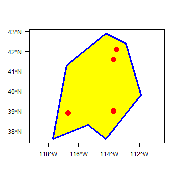
We’ll make more fancy maps later.