Local statistics
Introduction
This handout accompanies Chapter 8 in O’Sullivan and Unwin (2010).
LISA
Get the data
Read the Auckland data.
if (!require("rspatial")) remotes::install_github('rspatial/rspatial')
library(rspatial)
auck <- sp_data('auctb.rds')
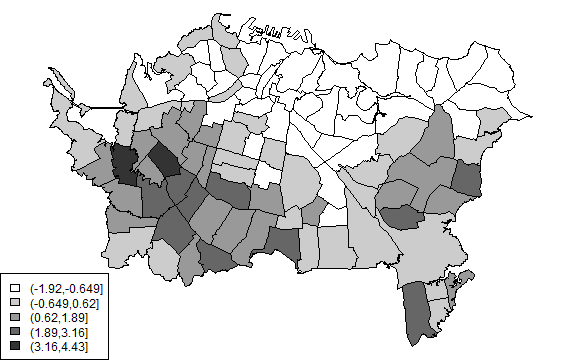
Local Getis Gi
library(spdep)
wr <- poly2nb(auck, row.names=auck$Id, queen=FALSE)
lstw <- nb2listw(wr, style='B')
Gi <- localG(auck$TB, lstw)
head(Gi)
## [1]  0.4241759  0.5623307  0.4047413  0.6819762 -1.3278352 -1.4086435
par(mai=c(0,0,0,0))
Gcuts <- cut(Gi, 5)
Gcutsi <- as.integer(Gcuts)
cols <- rev(gray(seq(0,1,.2)))
plot(auck, col=cols[Gcutsi])
legend('bottomleft', levels(Gcuts), fill=cols)
To get the Gi * we need to include each polygon as its own ‘neighbor’
ws <- include.self(wr)
lstws <- nb2listw(ws, style='B')
Gis <- localG(auck$TB, lstws)
Gscuts <- cut(Gis, 5)
Gscutsi <- as.integer(Gscuts)
cols <- rev(gray(seq(0,1,.2)))
plot(auck, col=cols[Gscutsi])
legend('bottomleft', levels(Gscuts), fill=cols)
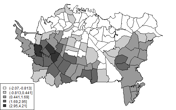
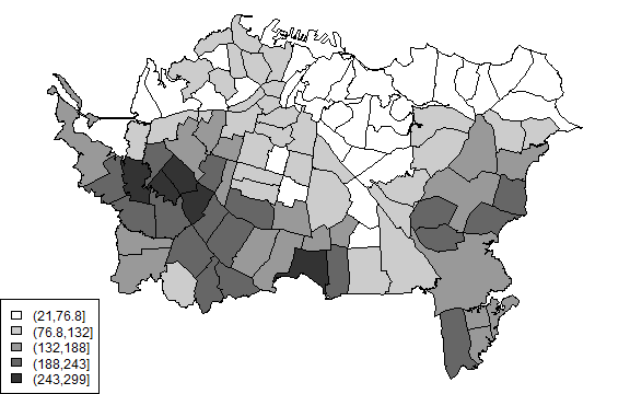
This looks very similar to the local average.
m <- sapply(ws, function(i) mean(auck$TB[i]))
cts <- cut(m, 5)
mcts <- as.integer(cts)
plot(auck, col=cols[mcts])
legend('bottomleft', levels(cts), fill=cols)
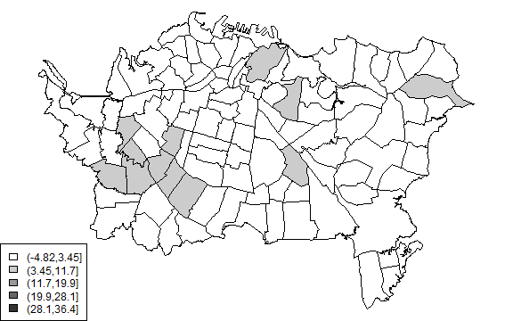
The local Moran Ii shows where there are locally high levels of autocorrelation.
Ii <- localmoran(auck$TB, lstw)
Icuts <- cut(Ii, 5)
Icutsi <- as.integer(Icuts)
plot(auck, col=cols[Icutsi])
legend('bottomleft', levels(Icuts), fill=cols)
Geographically weighted regression
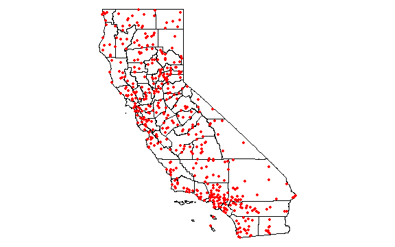
Here is an example of GWR with California precipitation data (you can download the data with the scripts or links on the top of this page).
cts <- sp_data('counties.rds')
p <- sp_data('precipitation.csv')
head(p)
##      ID                 NAME   LAT    LONG ALT  JAN FEB MAR APR MAY JUN JUL
## 1 ID741         DEATH VALLEY 36.47 -116.87 -59  7.4 9.5 7.5 3.4 1.7 1.0 3.7
## 2 ID743  THERMAL/FAA AIRPORT 33.63 -116.17 -34  9.2 6.9 7.9 1.8 1.6 0.4 1.9
## 3 ID744          BRAWLEY 2SW 32.96 -115.55 -31 11.3 8.3 7.6 2.0 0.8 0.1 1.9
## 4 ID753 IMPERIAL/FAA AIRPORT 32.83 -115.57 -18 10.6 7.0 6.1 2.5 0.2 0.0 2.4
## 5 ID754               NILAND 33.28 -115.51 -18  9.0 8.0 9.0 3.0 0.0 1.0 8.0
## 6 ID758        EL CENTRO/NAF 32.82 -115.67 -13  9.8 1.6 3.7 3.0 0.4 0.0 3.0
##    AUG SEP OCT NOV DEC
## 1  2.8 4.3 2.2 4.7 3.9
## 2  3.4 5.3 2.0 6.3 5.5
## 3  9.2 6.5 5.0 4.8 9.7
## 4  2.6 8.3 5.4 7.7 7.3
## 5  9.0 7.0 8.0 7.0 9.0
## 6 10.8 0.2 0.0 3.3 1.4
plot(cts)
points(p[,c('LONG', 'LAT')], col='red', pch=20)
Compute annual average precipitation
p$pan <- rowSums(p[,6:17])
Global regression model
m <- lm(pan ~ ALT, data=p)
m
##
## Call:
## lm(formula = pan ~ ALT, data = p)
##
## Coefficients:
## (Intercept)          ALT
##      523.60         0.17
Create Spatial* objects with a planar crs.
alb <- CRS("+proj=aea +lat_1=34 +lat_2=40.5 +lat_0=0 +lon_0=-120 +x_0=0 +y_0=-4000000 +ellps=GRS80 +datum=NAD83 +units=m +no_defs")
sp <- p
coordinates(sp) = ~ LONG + LAT
crs(sp) <- "+proj=longlat +datum=NAD83"
spt <- spTransform(sp, alb)
ctst <- spTransform(cts, alb)
## Warning in spTransform(xSP, CRSobj, ...): NULL source CRS comment, falling back
## to PROJ string
Get the optimal bandwidth
library( spgwr )
bw <- gwr.sel(pan ~ ALT, data=spt)
## Bandwidth: 526221.1 CV score: 64886883
## Bandwidth: 850593.6 CV score: 74209073
## Bandwidth: 325747.9 CV score: 54001118
## Bandwidth: 201848.6 CV score: 44611213
## Bandwidth: 125274.7 CV score: 35746320
## Bandwidth: 77949.39 CV score: 29181737
## Bandwidth: 48700.74 CV score: 22737197
## Bandwidth: 30624.09 CV score: 17457161
## Bandwidth: 19452.1 CV score: 15163436
## Bandwidth: 12547.43 CV score: 19452191
## Bandwidth: 22792.75 CV score: 15512988
## Bandwidth: 17052.67 CV score: 15709960
## Bandwidth: 20218.99 CV score: 15167438
## Bandwidth: 19767.99 CV score: 15156913
## Bandwidth: 19790.05 CV score: 15156906
## Bandwidth: 19781.39 CV score: 15156902
## Bandwidth: 19781.48 CV score: 15156902
## Bandwidth: 19781.47 CV score: 15156902
## Bandwidth: 19781.47 CV score: 15156902
## Bandwidth: 19781.47 CV score: 15156902
## Bandwidth: 19781.47 CV score: 15156902
bw
## [1] 19781.47
Create a regular set of points to estimate parameters for.
r <- raster(ctst, res=10000)
r <- rasterize(ctst, r)
newpts <- rasterToPoints(r)
Run the gwr function
g <- gwr(pan ~ ALT, data=spt, bandwidth=bw, fit.points=newpts[, 1:2])
g
## Call:
## gwr(formula = pan ~ ALT, data = spt, bandwidth = bw, fit.points = newpts[,
##     1:2])
## Kernel function: gwr.Gauss
## Fixed bandwidth: 19781.47
## Fit points: 4087
## Summary of GWR coefficient estimates at fit points:
##                    Min.    1st Qu.     Median    3rd Qu.      Max.
## X.Intercept. -702.40121   79.54254  330.48807  735.42718 3468.8702
## ALT            -3.91270    0.03058    0.20461    0.41542    4.6133
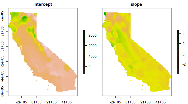
Link the results back to the raster
slope <- r
intercept <- r
slope[!is.na(slope)] <- g$SDF$ALT
intercept[!is.na(intercept)] <- g$SDF$'(Intercept)'
s <- stack(intercept, slope)
names(s) <- c('intercept', 'slope')
plot(s)
See this page for a more detailed example of Geographically weighted regression.